From 3:30-4:30pm Eastern Daylight Time every Wednesday, one of us will be at the computer to answer your questions. At those times, please video call us via Google Hangout at fragilefamilieschallenge@gmail.com.
Despite coming from disadvantaged backgrounds, some kids manage to “beat the odds” and achieve unexpectedly positive outcomes. Meanwhile, other kids who seem on track sometimes struggle unexpectedly. Policymakers would like to know what variables are associated with “beating the odds” since this could generate new theories about how to help future generations of disadvantaged children.
Once we combine all of the submissions to the Fragile Families Challenge into one collaborative guess for how children will be doing on each outcome at age 15, we will identify a small number of children doing much better than expected (“beating the odds”), and another set who are doing much worse than expected (“struggling unexpectedly”). By interviewing these sets of children, we will be well-positioned to learn what factors were associated with who ended up in each group.
What we learn in these interviews will affect the questions asked in future waves of the Fragile Families Study, and possibly other studies like it. By combining quantitative models with inductive interviews, the Fragile Families Challenge offers a new way to improve surveys in the future and expand the range of social science theories. In the remainder of this blog, we discuss current approaches to survey design and the potential contribution of the Fragile Families Challenge.
Deductive survey design: Evaluating theories
Social scientists often design surveys using deductive approaches based on theoretical perspectives. For instance, economists theorize about how one’s employment depends on the hypothetical wage offer (often called a “reservation wage”) one would have to be given before one would leave other unpaid options behind and opt into paid labor. Motivated by this theoretical perspective, Fragile Families and other surveys have incorporated questions like: “What would the hourly wage have to be in order for you to take a job?”
However, even the best theoretically-informed social science measures perform poorly at the task of predicting outcomes. R-squared, a measure of a model’s predictive validity, often ranges from 0.1 to 0.3 in published social science papers. Simply put, a huge portion of the variance in outcomes we care about is unexplained by the predictors social scientists have invented and put their faith in.
Inductive interviews: A source of new hypotheses
How can we be missing so much? Part of the problem might be that academics who propose these theoretical perspectives often spend their lives far from the context in which the data are actually collected. An alternative, inductive approach is to conduct open-ended interviews with interesting cases and allow the theory to emerge from the data. This approach is often used in ethnographic and other qualitative work, and points researchers toward alternative perspectives they never would have considered on their own.
Inductive approaches have their drawbacks: researchers might develop a theory that works well for some children, but does not generalize to other cases. Likewise, the unmeasured factors we discover will not necessarily be causal. However, inductive interviews will generate hypotheses that can be later evaluated using deductive approaches in new datasets, and finally evaluated with randomized controlled trials.
An ideal combination: Cycling between the two
To our knowledge, the Fragile Families Challenge is the first attempt to cycle between these two approaches. The study was designed with deductive approaches: researchers asked questions based on social science theories about the reproduction of disadvantage. However, we can use qualitative interviews to inductively learn new variables that ought to be collected. Finally, we will incorporate these variables in future waves of data collection to deductively evaluate theories generated in the interviews, using out-of-sample data.
By participating in the Fragile Families Challenge, you are part of a scientific endeavor to create the surveys of the future.
discusses how missing data is coded in the Fragile Families study
offers a brief theoretical introduction to the statistical challenges of missing data
links to software that implements one solution: multiple imputation
Of course, you can use any strategy you want to deal with missing values: multiple imputation is just one strategy among many.
Missing data in the Fragile Families study
Missing data is a challenge in almost all social science research. It generally comes in two forms:
Item non-response: Respondents simply refuse to answer a survey question.
Survey non-response: Respondents cannot be located or refuse to answer any questions in an entire wave of the survey.
While the first problem is common in any dataset, the second is especially prevalent in panel studies like Fragile Families, in which the survey is composed of interviews conducted at various child ages over the course of 15 years.
While the survey documentation details the codes for each variable, a few global rules summarize the way missing values are coded in the data. The most common responses are bolded.
-9 Not in wave – Did not participate in survey/data collection component
-8 Out of range – Response not possible; rarely used
-7 Not applicable (also -10/-14) – Rarely used for survey questions
-6 Valid skip – Intentionally not asked question; question does not apply to respondent or response known based on prior information.
-5 Not asked “Invalid skip” – Respondent not asked question in the version of the survey they received.
-3 Missing – Data is missing due to some other reason; rarely used
-1 Refuse – Respondent asked question; Refused to answer question
When responses are coded -6, you should look at the survey questionnaire to determine the skip pattern. What did these respondents tell us in prior questions that caused the interviewer to skip this question? You can then decide the correct way to code these values given your modeling approach.
When responses are coded -9, you should be aware that many questions will be missing for this respondent because they missed an entire wave of the survey.
For most other categories, an algorithmic solution as described below may be reasonable.
Theoretical issues with missing data
Before analyzing data with missing values, researchers must make assumptions about how some data came to be missing. One of the most common assumptions is the assumption that data are missing at random. For this assumption to hold, the pattern of missingness must be a function of the other variables in the dataset, and not a function of any unobserved variables once those observed are taken into account.
For instance, suppose children born to unmarried parents are less likely to be interviewed at age 9 than those born to married parents. Since the parents’ marital status at birth is a variable observed in the dataset, it is possible to adjust statistically for this problem. Suppose, on the other hand, that some children miss the age 9 interview because they suddenly had to leave town to attend the funeral of a their second cousin once removed. This variable is not in the dataset, so no statistical adjustment can fully account for this kind of missingness.
For a full theoretical treatment, we recommend
One solution: Imputation
Once we assume that data are missing at random, a valid approach to dealing with the missing data is imputation. This is a procedure whereby the researcher estimates the association between all of the variables in the model, then fills in (“imputes”) reasonable guesses for the values of the missing variables.
The simplest version of imputation is known as single imputation. For each missing value, one would use an algorithm to guess the correct value for every missing observation. This produces one complete dataset, which can be analyzed like any other. However, single imputation fails to account for our uncertainty about the true values of the missing cases.
Multiple imputation is a procedure that produces several data sets (often in the range of 5, 10, or 30), with slightly different imputed values for the missing observations in each data set. Differences across the datasets capture our uncertainty about the missing values. One can then estimate a model on each imputed dataset, then combine estimates across the imputed datasets using a procedure known as Rubin’s rules.
Ideally, one would conduct multiple imputation on a dataset with all of the observed variables. In practice, this can become computationally intractable in a dataset like Fragile Families with thousands of variables. In practice, researchers often select the variables to be included in their model, restrict the data to only those variables, and then multiply impute missing values in this subset.
Implementing multiple imputation
There are many software packages to implement multiple imputation. A few are listed below.
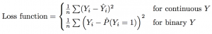
We will evaluate submissions based on predictive validity, measured in the held-out test data by mean squared error loss for continuous outcomes and Brier loss for binary outcomes.
A leaderboard will rank submissions according to these criteria, using a set of held-out data. After the challenge closes, we will produce a finalized ranking of submissions based on a separate set of withheld true outcome data.
Each of the 6 outcomes will be evaluated and ranked independently – feel free to focus on predicting one outcome well!
What does this mean for you?
You should produce a submission that performs well out of sample. Mean squared error is a function of both bias and variance. A linear regression model with lots of covariates is an unbiased predictor, but it might overfit the data and produce predictions that are highly sensitive to the sample used for training. Computer scientists often refer to this problem as the challenge of distinguishing the signal from the noise; you want to pick up on the signal in the training data without picking up on the noise.
An overly simple model will fail to pick up on meaningful signal. An overly complex model will pick up too much noise. Somewhere in the middle is a perfect balance – you can help us find it!
The Fragile Families Challenge presents a unique opportunity to probe the assumptions required for causal inference with observational data. This post introduces these assumptions and highlights the contribution of the Fragile Families Challenge to this scientific question.
Causal inference: The problem
Social scientists and policymakers often wish to use empirical data to infer the causal effect of a binary treatment D on an outcome Y. The causal effect for each respondent is the potential outcome that each observation would take under treatment (denoted Y(1)) minus the potential outcome that each observation would take under control (denoted Y(0)). However, we immediately run into the fundamental problem of causal inference: each observation is observed either under the treatment condition or under the control condition.
The solution: Assumptions of ignorability
The gold standard for resolving this problem is a randomized experiment. By randomly assigning treatment, researchers can ensure that the potential outcomes are independent of treatment assignment, so that the average difference in outcomes between the two groups can only be attributable to treatment. This assumption is formally called ignorability.
Ignorability:{Y(0),Y(1)} 丄 D
Because large-scale experiments are costly, social scientists frequently draw causal inferences from observational data based on a simplifying assumption of conditional ignorability.
Conditional ignorability: {Y(0),Y(1)} 丄 D | X
Given a set of covariates X, conditional ignorability states that treatment asignment D is independent of the potential outcomes that would be realized under treatment Y(1) and control Y(0). In other words, two observations with the same set of covariates X but with different treatment statuses can be compared to estimate the causal effect of the treatment for these observations.
Assessing the credibility of the ignorability assumption
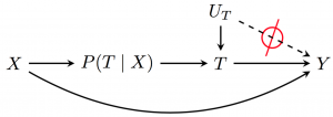
Conditional ignorability is an enormous assumption, yet it is what the vast majority of social science findings rely on. By writing the problem in a Directed Acyclic Graph (DAG, Pearl 2000), we can make the assumption more transparent.
X represents pre-treatment confounders that affect both the treatment and the outcome. Though it is not the only way to do so, researchers often condition on X by estimating the probability of treamtent given X, denoted P(T | X). Once we account for the differential probability of a treatment by the background covariates (through regression, matching, or some other method), we say we have blocked the noncausal backdoor paths connecting T and Y through X.
The key assumption in the left panel has to do with Ut. We assume that all unobserved variables that affect the treatment (Ut) have no affect on the outcome Y, except through T. This is depicted graphically by the dashed line from Ut to Y, which we must assume does not exist for causal inferences to be valid.
Researchers often argue that conditional ignorability is a reasonable assumption if the set of predictors included in X is extensive and detailed. The Fragile Families Challenge is an ideal setting in which to test the credibility of this assumption: we have a very detailed set of predictor variables X collected from birth through age 9, which occur temporally prior to treatments reported at age 15.
Nevertheless, the assumption of conditional ignorability is untestable. Interviews may provide some insight to the credibility of this assumption.
Goal of the Fragile Families Challenge: Targeted interviews
Through targeted interviews with particularly informative children, we might be able to learn something about the plausibility of the conditional ignorability assumption.
One of the binary variables in the Fragile Families Challenge is whether a child was evicted from his or her home. We will treat this variable as T. We want to know the causal effect of eviction on a child’s chance of graduating from high school (Y). In the Fragile Families Challenge, the set of observed covariates X is all 12,000+ predictor variables included in the Fragile Families Challenge data file.
Based on the ensemble model from the Fragile Familie Challenge, we will identify 20 children who were evicted, and 20 similar children who had similar predicted probabilities of eviction but were not evicted. We will interview these children to find out why they were evicted.
Potential interviews in support of conditional ignorability:
Suppose we find that children were evicted because their landlords were ready to retire and wanted to get out of the housing market. Those who were not evicted had younger landlords. It might be plausible that the age of one’s landlord is an example of Ut: a variable that affects eviction but has no effect on high school graduation except through eviction. While this would not prove the conditional ignorability assumption, the assumption might seem reasonable in this case.
Potential interviews that discredit conditional ignorability:
Suppose instead that we find a different story. Gang activity increased in the neighborhoods of some families, escalating to the point that landlords decided to get out of the business and evict all of their tenants. Other families lived in neighborhoods with no gang activity, and they were not evicted. In addition to its effect on eviction, it is likely that gang activity would alter the chances of high school graduation in other ways, such as by making students feel unsafe at school. In this example, gang activity plays the role of Uty and would violate the assumption of conditional ignorability.
Summary
Because costs prohibit randomized experiments to evaluate all potential treatments of interest to social scientists, scholars frequently rely on the assumption of conditional ignorability to draw causal claims from observational data. This is a strong and untestable assumption. The Fragile Families Challenge is a setting in which the assumption may be plausible, due to the richness of the covariate set X, which includes over 12,000 pre-treatment variables chosen for their potentially important ramifications for child development.
By interviewing a targeted set of children chosen by ensemble predictions of the treatment variables, we will shed light on the credibility of the ignorability assumption.
This post will walk you through the steps to prepare your files for submission and upload them to the submission platform. The organizer of your group (i.e. your professor or TA) will provide a link to the submission platform.
1. Save your predictions as prediction.csv.
This file should be structured the same way as the “prediction.csv” file provided as part of your data bundle.
This file should have 4,242 rows: one for each observation in the test set.
We are asking you to make predictions for all 4,242 cases, which includes both the training cases from train.csv and the held-out test cases. We would prefer that you not simply copy these cases from train.csv to prediction.csv. Instead, please submit the predictions that come out of your model. This way, we can compare your performance on the training and test sets, to see whether those who fit closely to the training set perform more poorly on the test set (see our blog discussing overfitting). Your scores will be determined on the basis of test observations alone, so your predictions for the cases included in train.csv will not affect your score.
There are some observations that are truly missing: we do not have the true answer for these cases because respondents did not complete the interview or did not answer the question. This is true for both the training and the test sets. Your predictions for these cases will not affect your scores. We are asking you to make predictions for missing cases because it is possible that we will find those respondents sometime in the future and uncover the truth. It will be scientifically interesting to know how well the community model was able to predict these outcomes which even the survey staff did not know at the time of the Challenge.
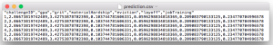
This file should have 7 columns for the ID number and the 6 outcomes. They should be named:
The top of the file will look like this (numbers here are random). challengeID numbers can be in any order.
2. Save your code.
3. Create a narrative explanation of your study. This should be saved in a file called “narrative” and can be a text file, PDF, or Word document.
At the top of this narrative explanation, tell us your names of everyone on the team that produced the submission, or your name if you worked alone, in the format:
Homer Simpson,
homer@gmail.com
Marge Simpson,
msimpson@gmail.com
Then, tell us about how you developed the submission. This might include your process for preparing a the data for analysis, methods you used in the analysis, how you chose the submission you settled on, things you learned, etc.
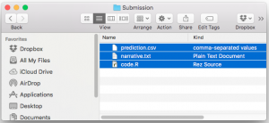
4. Zip all the files together in one folder.
It is important that the files be zipped in a folder with no sub-directories. Instructions are different for Mac and windows.
On Mac, highlight all of the individual files.
Right click and choose “Compress 3 items”.
On Windows, highlight all of the individual files.
Right click and choose
Send to -> Compressed (zipped) folder
5. Upload the zipped folder to the submission site. The link to this will be provided to you by the organizers (i.e. your professor or TA) of your specific instance of the Fragile Families Challenge.
Click the “Participate” tab at the top, then the “Submit / View Results” tab on the left. Click the “Submit” button to upload your submission.
6. Wait for the platform to evaluate your submission.
Click “Refresh status” next to your latest submission to view its updated status and see results when they are ready. If successful, you will automatically be placed on the leaderboard when evaluation finishes.
Take our data and build models for the 6 child outcomes at age 15. Your model might draw on social science theories about variables that affect the outcomes. It might be a black-box machine learning algorithm that is hard to interpret but performs well. Perhaps your model is some entirely new combination no one has ever seen before!
The power of the Fragile Families Challenge comes from the heterogeneity of quality individual models we receive. By working together, we will harness the best of a range of modeling approaches. Be creative and show us how well your model can perform!
You can try them all and then choose the best one! Our submission platform allows you to upload up to 10 submissions per day. Submissions will instantly be scored, and your most recent submission will be placed on the leaderboard. If you have several ideas, we suggest you upload them each individually and then upload a final submission based on the results of the individual submissions.
What if I don’t have time to make 6 models?
You can make predictions for whichever outcome interests you. To upload a submission with the appropriate file size, make a simple numeric guess for the rest of the outcomes. For instance, you might develop a careful model for grit, and then guess the mean of the training values for all of the remaining five observations. This would still allow you to upload 6 sets of predictions to the scoring function.
The Fragile Families Challenge is now closed. We are no longer accepting applications!
What will happen after I apply?
We will review your application and be in touch by e-mail. This will likely take 2-3 business days. If we invite you to participate, you will be asked to sign a data protection agreement. Ultimately, each participant will be given a zipped folder which consolidates all of the relevant pieces of the larger Fragile Families and Child Wellbeing Study in three .csv files.
background.csv contains 4,242 rows (one per child) and 12,943 columns:
challengeID: A unique numeric identifier for each child.
12,942 background variables asked from birth to age 9, which you may use in building your model.
train.csv contains 2,121 rows (one per child in the training set) and 7 columns:
challengeID: A unique numeric identifier for each child.
Six outcome variables (each variable name links to a blog post about that variable)
Continuous variables: grit, gpa, materialHardship
Binary variables: eviction, layoff, jobTraining
prediction.csv contains 4,242 rows and 7 columns:
challengeID: A unique numeric identifier for each child.
Six outcome variables, as in train.csv. These are filled with the mean value in the training set. This file is provided as a skeleton for your submission; you will submit a file in exactly this form but with your predictions for all 4,242 children included.
Understanding the background variables
To use the data, it may be useful to know something about what each variable (column) represents. Full documentation is available here, but this blog post distills the key points.
Waves and child ages
The background variables were collected in 5 waves.
Wave 1: Collected in the hospital at the child’s birth.
Wave 2: Collected at approximately child age 1
Wave 3: Collected at approximately child age 3
Wave 4: Collected at approximately child age 5
Wave 5: Collected at approximately child age 9
Note that wave numbers are not the same as child ages. The variable names and survey documentation are organized by wave number.
Variable naming conventions
Predictor variables are identified by a prefix and a question number. Prefixes the survey in which a question was collected. This is useful because the documentation is organized by survey. For instance the variable m1a4 refers to the mother interview in wave 1, question a4.
The prefix c in front of any variable indicates variables constructed from other responses. For instance, cm4b_age is constructed from the mother wave 4 interview, and captures the child’s age (baby’s age).
m1, m2, m3, m4, m5: Questions asked of the child’s mother in wave 1 through wave 5.
f1,...,f5: Questions asked of the child's father in wave 1 through wave 5
hv3, hv4, hv5: Questions asked in the home visit in waves 3, 4, and 5.
p5: Questions asked of the primary caregiver in wave 5.
k5: Questions asked of the child (kid) in wave 5
ffcc: Questions asked in various child care provider surveys in wave 3