Author ilundberg

Author ilundberg

Privacy, ethics, and data access: A case study of the Fragile Families Challenge

Uncategorized 1 comment

This blog post summarizes a paper describing the privacy and ethics process by which we organized the Fragile Families Challenge. The paper will appear in a special issue of the journal Socius. This post is cross-posted on the Freedom to Tinker blog.

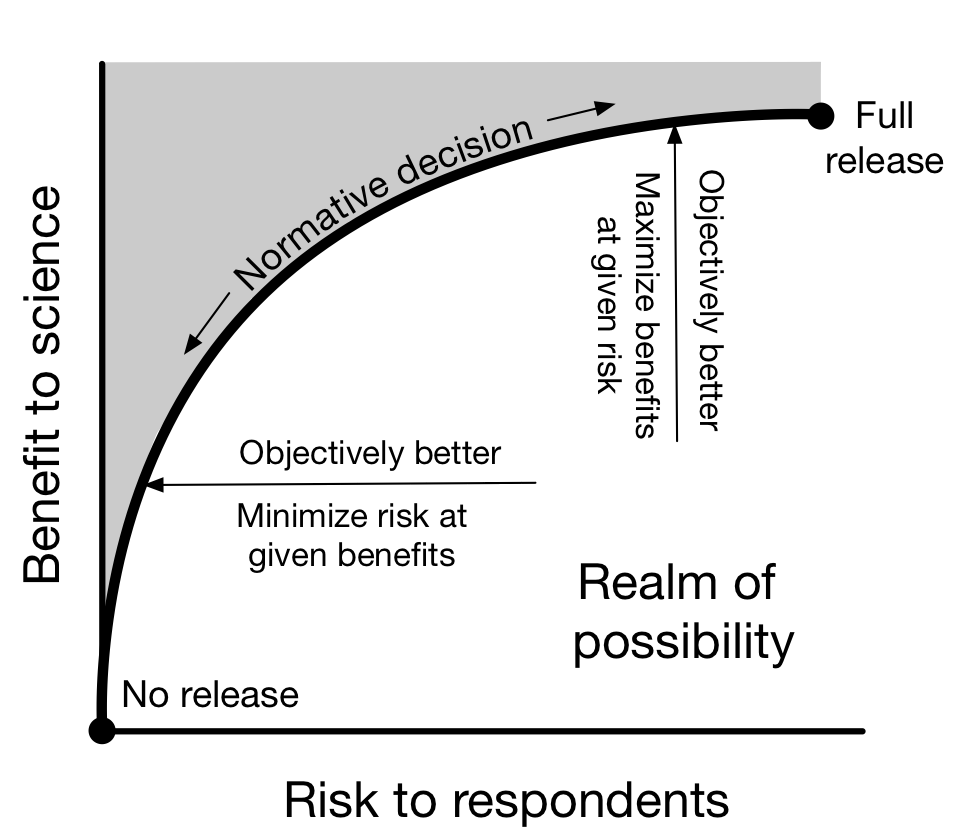
Academic researchers, companies, and governments holding data face a fundamental tension between risk to respondents and benefits to science. On one hand, these data custodians might like to share data with a wide and diverse set of researchers in order to maximize possible benefits to science. On the other hand, the data custodians might like to keep data locked away in order to protect the privacy of those whose information is in the data. Our paper is about the process we used to handle this fundamental tension in one particular setting: the Fragile Families Challenge, a scientific mass collaboration designed to yield insights that could improve the lives of disadvantaged children in the United States. We wrote this paper not because we believe we eliminated privacy risk, but because others might benefit from our process and improve upon it.

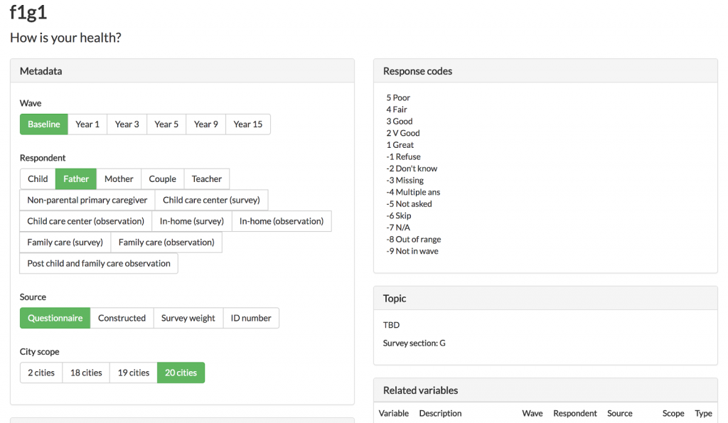
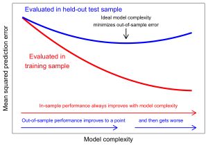
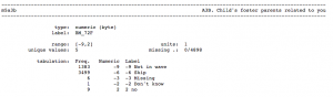
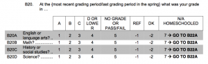
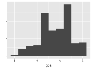
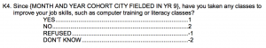
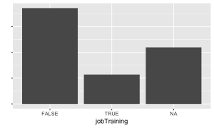
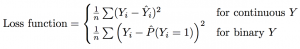
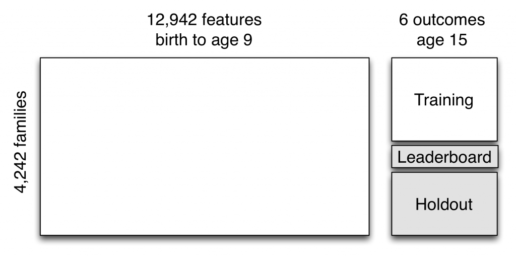
One scientific objective of the Fragile Families Challenge was to maximize predictive performance of adolescent outcomes (i.e. high school GPA) measured at approximately age 15 given a set of background variables measured from birth through age 9. We aimed to do so using the Common Task Framework (see Donoho 2017, Section 6): we would share data with researchers who would build predictive models using observed outcomes for half of the cases (the training set). These researchers would receive instant feedback on out-of-sample performance in ⅛ of the cases (the leaderboard set) and ultimately be evaluated by performance in ⅜ of the cases which we would keep hidden until the end of the Challenge (the holdout set). If scientific benefit was the only goal, the optimal design might be to include every possible variable in the background set and share with anyone who wanted access with no restrictions.

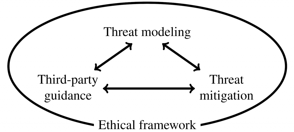
Scientific benefit may be maximized by sharing data widely, but risk to respondents is also maximized by doing so. Although methods of data sharing with provable privacy guarantees are an active area of research, we believed that solutions that could offer provable guarantees were not possible in our setting without a substantial loss of scientific benefit (see preprint section 2.4). Instead, we engaged in a privacy and ethics process that involved threat modeling, threat mitigation, and third-party guidance, all undertaken within an ethical framework.


Threat modeling

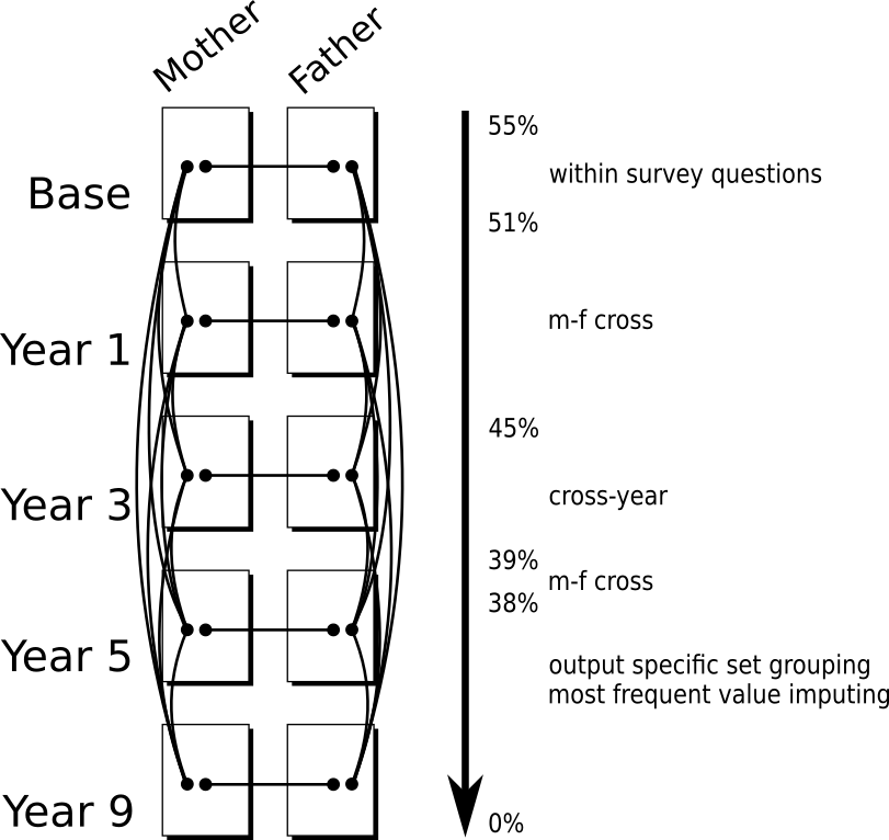
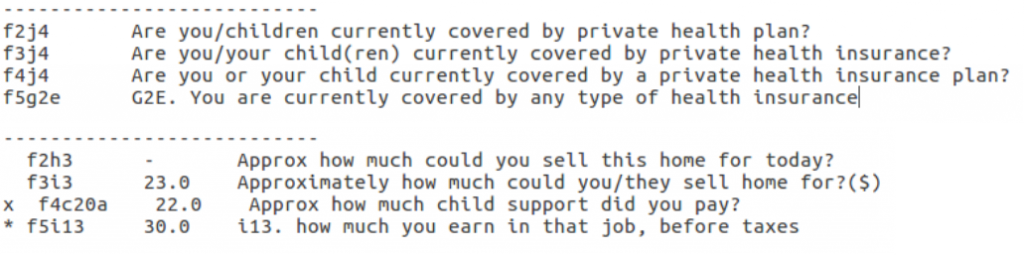
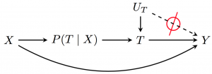
Our primary concern was a risk of re-identification. Although our data did not contain obvious identifiers, we worried that an adversary could find an auxiliary dataset containing identifiers as well as key variables also present in our data. If so, they could link our dataset to the identifiers (either perfectly or probabilistically) to re-identify at least some rows in the data. For instance, Sweeney (2002) was able to re-identify Massachusetts medical records data by linking to identified voter records using the shared variables zip code, date of birth, and sex. Given the vast number of auxiliary datasets (red) that exist now or may exist in the future, it is likely that some research datasets (blue) could be re-identified. It is difficult to know in advance which key variables (purple) may aid the adversary in this task.

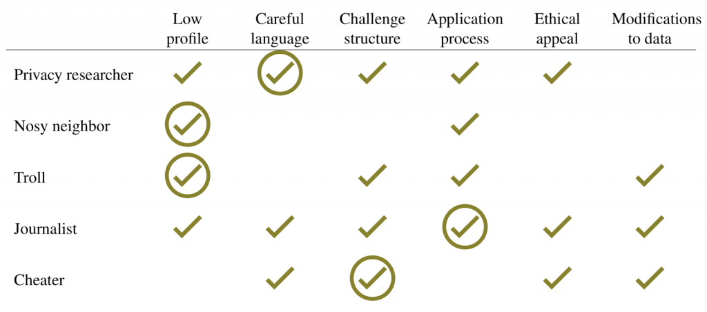
To make our worries concrete, we engaged in threat modeling: we reasoned about who might have both (a) the capability to conduct such an attack and (b) the incentive to do so. We even tried to attack our own data.  Through this process we identified five main threats (the rows in the figure below). A privacy researcher, for instance, would likely have the skills to re-identify the data if they could find auxiliary data to do so, and might also have an incentive to re-identify, perhaps to publish a paper arguing that we had been too cavalier about privacy concerns. A nosy neighbor who knew someone in the data might be able to find that individual’s case in order to learn information about their friend which they did not already know. We also worried about other threats that are detailed in the full paper.


Threat mitigation

To mitigate threats, we took several steps to (a) reduce the likelihood of re-identification and to (b) reduce the risk of harm in the event of re-identification. While some of these defenses were statistical (i.e. modifications to data designed to support aims [a] and [b]), many instead focused on social norms and other aspects of the project that are more difficult to quantify. For instance, we structured the Challenge with no monetary prize, to reduce an incentive to re-identify the data in order to produce remarkably good predictions. We used careful language and avoided making extreme claims to have “anonymized” the data, thereby reducing the incentive for a privacy researcher to correct us. We used an application process to only share the data with those likely to contribute to the scientific goals of the project, and we included an ethical appeal in which potential participants learned about the importance of respecting the privacy of respondents and agreed to use the data ethically. None of these mitigations eliminated the risk, but they all helped to shift the balance of risks and benefits of data sharing in a way consistent with ethical use of the data. The figure below lists our main mitigations (columns), with check marks to indicate the threats (rows) against which they might be effective.  The circled check mark indicates the mitigation that we thought would be most effective against that particular adversary.


Third-party guidance

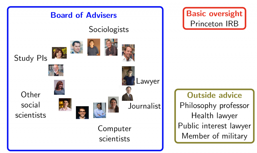
A small group of researchers highly committed to a project can easily convince themselves that they are behaving ethically, even if an outsider would recognize flaws in their logic. To avoid groupthink, we conducted the Challenge under the guidance of third parties. The entire process was conducted under the oversight and approval of the Institutional Review Board of Princeton University, a requirement for social science research involving human subjects. To go beyond what was required, we additionally formed a Board of Advisers to review our plan and offer advice. This Board included experts from a wide range of fields.

Beyond the Board, we solicited informal outside advice from a diverse set of anyone we could talk to who might have thoughts about the process, and this proved valuable.  For example, at the advice of someone with experience planning high-risk operations in the military, we developed a response plan in case something went wrong. Having this plan in place meant that we could respond quickly and forcefully should something unexpected have occurred.


Ethics

After the process outlined above, we still faced an ethical question: should we share the data and proceed with the Fragile Families Challenge? This was a deep and complex question to which a fully satisfactory answer was likely to be elusive. Much of our final decision drew on the principles of the Belmont Report, a standard set of principles used in social science research ethics. While not perfect, the Belmont Report serves as a reasonable benchmark because it is the standard that has developed in the scientific community regarding human subjects research. The first principle in the Belmont Report is respect for persons. Because families in the Fragile Families Study had consented for their data to be used for research, sharing the data with researchers in a scientific project agreed with this principle. The second principle is beneficence, which requires that the risks of research be balanced against potential benefits. The threat mitigations we carried out were designed with beneficence in mind. The third principle is justice: that the benefits of research should flow to a similar population that bears the risks. Our sample included many disadvantaged urban American families, and the scientific benefits of the research might ultimately inform better policies to help those in similar situations. It would be wrong to exclude this population from the potential to benefit from research, so we reasoned that the project was in line with the principle of justice. For all of these reasons, we decided with our Board of Advisers that proceeding with the project would be ethical.


Conclusion

To unlock the power of data while also respecting respondent privacy, those providing access to data must navigate the fundamental tension between scientific benefits and risk to respondents. Our process did not offer provable privacy guarantees, and it was not perfect. Nevertheless, our process to address this tension may be useful to others in similar situations as data stewards. We believe the core principles of threat modeling, threat mitigation, and third-party guidance within an ethical framework will be essential to such a task, and we look forward to learning from others in the future who build on what we have done to improve the process of navigating this tension.

You can read more about our process in our pre-print: Lundberg, Narayanan, Levy, and Salganik (2018) “Privacy, ethics, and data access: A case study of the Fragile Families Challenge.”

Scientific Workshop Breakout Sessions

Uncategorized No comments

At the Fragile Families Challenge Scientific Workshop, we devoted Thursday afternoon to breakout sessions where participants could work on specific projects that grew out of the Challenge. In this blog post we’d like to describe what happened in the breakout sessions, what we learned, and what is going to happen going forward.

Demo for the new Fragile Families metadata API and front-end (led by Maya Phillips and Alex Kindel)

Background: One of the things that we discovered during the Challenge is that much of the metadata about the Fragile Families study is stored in pdf files of codebooks that are designed to be read by people and are not designed to be machine-actionable (in the sense that they are easy to process with code). During the Challenge, one of the participants—Gregory Gundersen—converted some of the existing documentation into a metadata API. We loved his idea so much that the Board awarded him the Foundational Prize, and we decided to try to build on what he did by creating more metadata, a more fully featured API, and a web front-end for the API.

The API workshop began with a brief presentation about the interface proof-of-concept, its intended audience, and the different design decisions that we made along the way. Participants provided positive feedback, which gave us confidence in our design decisions. We determined that providing an API independent of the front-end enables the widest audience to make use of the data: both for more technical users invoking the API directly and for less technical users relying on the guided functionality of the front-end. The workshop proceeded to discuss some of the core functionality before doing a brief code walkthrough and demonstration of the front-end’s main features.

API discussion led by Maya Phillips and Alex Kindel

Discussing the different API functions helped to affirm the idea that complex queries could be created by chaining simple functions together (e.g. search variables, display variable). Therefore, we will build a few simple functions that are designed to fit together, rather than many specific functions for different use cases. For example, we plan to enable Boolean searches over the metadata fields, making it possible to quickly combine multiple searches. We also discussed the different ways queries can be made to the API: through a local copy, through Python or R libraries, or through web requests to a remote server. Providing a web server presents some trade-offs (e.g. between consistency guarantees and query speed), so we sought feedback on how users might think about this tradeoff. Given that the typical use case will involve only a couple of queries, we determined that consistency was more important than query speed, but we intend to provide a full CSV copy of the metadata in the event that researchers need to perform more intensive metadata analysis.

Participants were hesitant about the use of PHP to implement the API. Although we initially chose PHP for the backend in order to coordinate with local web development and maintenance resources at Princeton, the workshop attendees stressed the importance of a community-maintainable and open-source code base to which others could add useful features and make updates as the technologies advance. Moving forward, we intend to use a modern web stack to design the API and front-end for the revised metadata. It seems that this is critically important to those who will be using the API in the future, and is the most in line with the vision the team has for the project moving forward.

Workshop participants were generally enthusiastic about the demo version of the metadata browser front-end. The demo was designed to prototype interactions with the basic features of the API. The group had several feature requests for the web interface, primarily revolving around search:

  1. An option to save and aggregate multiple searches
  2. An option to copy and paste metadata (especially variable names) directly into code
  3. Logging user queries to provide the FFCWS community with additional information on which variables are being used
  4. Supplying data users with more information on possible responses, especially missing values
  5. Displaying additional information on variable groups in the search interface
  6. Naming queries to provide easy, commonly used shortcuts into the search interface
  7. Enabling search over all data fields, including tags and responses

We intend to implement several of these features before the public launch of the website.


Figure 1. Variable browser search interface at the time of the workshop.


Figure 2. Variable metadata page at the time of the workshop.

Maya will continue to develop the back-end codebase by doing rigorous testing and adding features that will support the new features requested on the front-end. Alex and Maya will continue to work closely together as they build and integrate this architecture. In particular, a near-term goal is to identify and implement a relational schema for storing a canonical copy of the metadata; this database will serve the API, which in turn will serve the front-end and related software packages.

Testing and improving the Docker container that ensure reproducibility of the special issue of Socius (led by David Liu)

Background: One of the goals of the Fragile Families Challenge is to help promote a culture of open and reproducible research. Therefore, we required all participants in the Challenge to open source their submissions (code, predictions, and narrative explanations). This does not, however, ensure that it is easy for future researchers to reproduce the results of any of the Challenge submissions because we never checked that the code actually ran and future researchers may lack the appropriate dependencies to get the code to run. Therefore, for all the manuscripts in the special issue of Socius, we are ensuring reproducibility by re-running the code as part of the review process and packaging up the code and all the necessary dependencies in Docker containers that will make it easy for future researchers to download and run the code used in the papers in the special issue.

The reproducibility session began with a brief presentation of the project’s motivations and progress thus far. In addition to discussing the working of Docker, David Liu discussed patterns he has noticed in submitted code as well as a few suggested best practices for reproducibility.
It was particularly helpful to explain the background of Docker containers to the audience. For some, the explanation clarified the technical workings; the questions David received helped him better anticipate potential areas of confusion, which will be useful when releasing the containers to the public. A useful take away from the discussion on Docker is that the reproducibility work stands at the intersection of both research and software engineering; many of the principles and best practices of software engineering are relevant to conducting reproducible research. Examples include writing code that modular, assembling documentation during development, and testing the code as it is being written.
Next, David walked through a demo of how an actual submission was reproduced. This demo was particularly fruitful because the author of the submission (Tom Davidson) was in the audience and provided helpful commentary regarding his submission, which utilized neural networks. The demo illustrated how one would run Docker on Amazon Web Services and interact with the code. One of the undergraduates in attendance was able to follow the demo.
Overall, the session reinforced the community’s interest in viewing the open-sourced submissions. It was apparent that submitters were curious to see how others developed and implemented their models, beyond just the results themselves. In discussing and critiquing the code itself, we were able to better understand the author’s intentions and learn from their code development process. So reproducing and publicly publishing the code will satisfy a research need.
Looking ahead, David is reaching completion with five of the thirteen submissions written in Python and R, and he intends on completing the reproducibility work over the course of December and January. In the end, David will open source Docker containers for each of the journal’s models and include basic documentation regarding usage of the code. In addition, David will be able to provide recommendations for future social research software development to optimize code reproducibility. Finally, David can provide tips and guidelines for other journal editors on how to best reproduce journal submissions while also establishing a baseline for expected time commitment.

David Liu leading a discussion about reproducibility.

Assessing test-retest reliability of concept tags (led by Kristin Catena)

Background: One of the difficulties that participants encountered during the Challenge was selecting from the many, many survey questions that were available. Several participants asked us for a list of all questions related to education, for example. Such a list was not available. Therefore, we are now tagging all variables in the dataset with the social science concepts that they are attempting to measure.

As part of our new work on the FFCWS metadata infrastructure, we are adding a system of concept tags to the FFCWS variables so that users may more easily identify a list of variables related to a particular topic. For example, the concept tags would allow a data user to quickly identify all of the variables related to mental health or all the variables related to child support. It would also mark variables that are considered paradata – data that is about the survey administration but may not contain substantive information about the family (e.g., survey date, whether a particular participant completed a specific survey, etc.). Each variable will be assigned one or more concept tag(s) which will also be grouped into larger “umbrella” concepts. For example, mental health will be grouped under an umbrella of health while child support will be grouped under an umbrella of finances. When complete, the concept tags will be available through the metadata API and website (described above).

At the Fragile Families Challenge Scientific Workshop, we held a breakout session to test and discuss the concept tag system. Each participant was given a questionnaire to code into a provided list of tags. We also saved time afterwards to discuss the process and list of tags. In general, the participants reported that the concept tag list would be very helpful to data users and that they thought the list includes the concepts they would hope to search for. Several participants from data science backgrounds noted that they thought the umbrella concepts would be very helpful for orienting their work as they got started, but that the specific concept tags would be less helpful for them. Participants with more of a social science background, on the other hand, were interested in both the umbrella concepts and specific concept tags.
After the workshop, the participants’ tags were compared with those assigned by content experts from the FFCWS staff. 205 variables from four different FFCWS surveys were each coded by a member of the FFCWS staff and two different participants of the workshop breakout session. 95% of all variables coded had at least one tester who tagged the variable with the same concept as the FFCWS staff. Further, in 60% of all cases the FFCWS staff and both testers applied the same tag to the variable. Only 11 of the 205 variables had zero agreement between testers and FFCWS staff. We are now reviewing these results to strengthen and clarify the list of concept tags before completing the process of assigning tags to all remaining FFCWS variables.

Garrett Pace tagging variables with concept tags

Ian Lundberg tagging variables with concept tags

Steve McKay tagging variables with concept tags

Liberating question and answer texts from pdfs (led by Tom Hartshorne)

Background: As described above, one of the lessons from the Challenge was that we wanted to make more of the metadata available in machine-actionable formats. One example of this is the actual text of the survey questions. Right now, that information is currently in many different pdf files, which makes it cumbersome to search efficiently. Therefore, we want to make it easier for people to search and process the exact text of each question.

The goal of this project was to extract the exact text of the questionnaires out of PDF form and into a machine readable csv formatted file. This would allow future researchers to efficiently locate questions that have a certain keyword in either the question itself or the possible responses. It would also allow for our API and website (described above) to return the exact wording of the question associated with a particular variable.

Tom Hartshorne pitched the question text task to the group

Prior to the workshop, a procedure was iteratively developed to extract the text manually, but this proved time consuming. One of the goals going into the workshop was to use the collective expertise of the community to try and develop an automated way of scraping these PDF’s. During the workshop’s afternoon breakout session, Tom Hartshorne introduced the problem to a group of Challenge participants. Some members of the group worked to sharpen the manual process by going through it themselves and pointing out additional information stored in the questionnaires that could be useful to researchers. For example, Nicole Carnegie proposed adding the skip pattern associated with each answer choice. This is something that had come up in her Challenge experience, but had not been considered by the Fragile Families team prior to the Workshop. The manual process was very helpful for understanding the nuances of the questionnaires such as the string of periods between each answer choice, the formatting of “Circle all that apply” questions, and the location of the skip pattern information.

Question text working group led by Tom Hartshorne

While some of the group worked on the manual process, others worked towards a possible automation of the process. Cambria Naslund led this group of members, writing a Python script that parses an HTML version of the questionnaire to liberate the question text. This code strips the variables of their prefixes, then searches the questionnaire for a matching name. Once it finds a match, it grabs all the text following the first paragraph break up to the last paragraph break before the next question. It then cleans up this text, separating the answers from the question text using the long string of periods found between each answer choice. Each of these answers is stored in its own column, along with any skip patterns that may be associated with that answer choice. The output of this code will still require some manual cleaning, but it should greatly shorten the manual effort required by this task. We’ve now moved the software development to GitHub.

Conclusion

Overall, it was a very productive afternoon. We want to again thank everyone that participated.

Leah Gillion talking with Sara McLanahan

Coffee was available in abundance

Media coverage of the Fragile Families Challenge by Princeton University

Uncategorized No comments

The Fragile Families Challenge has been featured in a post by the Princeton University Office of Communications. Read about where we are and what we’ve learned so far!

We also held a scientific workshop on the Fragile Families Challenge Nov. 16-17 at Princeton University. Many participants came and we have learned a lot about the models submitted to the Challenge. Watch the blog for a video link coming soon with recordings from the workshop!

MDRC’s Approach to the Fragile Families Challenge

Uncategorized No comments

Guest post by Kristin E. Porter, Tejomay Gadgil, Sara Schell, Megan McCormick and Richard Hendra, MDRC.

Predictive analytics at MDRC

For more than 40 years, MDRC, a nonprofit, nonpartisan education and social policy research organization, has been a leader in pioneering the most rigorous research methods in social science research and in sharing what we have learned with the field. In this blog post, we describe how MDRC’s rigorous approach to methodology and data processing is reflected in our approach to predictive analytics, which we believe led to our first place performance in the two Fragile Families Challenge domains where we submitted models.

MDRC works with a wide variety of government agencies, nonprofits, and other social service providers to help them harness their data to better understand patterns of behavior, figure out what works, better manage caseload dynamics, and better target individuals for interventions. In particular, we are using predictive analytics to identify individuals’ likelihoods of achieving key outcomes, such as reaching a program participation milestone, finding employment, or reading at a proficient level.

MDRC researchers have developed a comprehensive predictive analytics framework that allows for rapid and iterative estimation of likelihoods (probabilities between 0 and 1) of adverse or positive outcomes. The framework includes analytic steps focused on (1) identifying the best samples for training statistical models and computing predictions; (2) processing and cleaning data; (3) creating and curating measures to include in modeling; (4) identifying the best modeling methods with an emphasis on ensembling; (5) estimating uncertainty in predictions; and (6) summarizing and interpreting results.

MDRC’s approach to the Fragile Families Challenge.

MDRC applied several analytic steps in our predictive analytics framework to the Fragile Families Challenge (FFC) — those focused on data processing, creating and curating measures, and modeling methods. (The other steps simply did not apply given the nature of the challenge.) The following describes the underlying premises that guided our analyses:

1. Invest deeply in measure creation — combining both substantive knowledge and automated approaches.

At MDRC, about 90 percent of the effort in any predictive analysis is dedicated to creating measures that extract as much predictive information as possible from the raw data. Doing so requires both subject matter expertise and familiarity with the data collection processes and context. It also involves recognizing opportunities for encoding information that may seem irrelevant or ancillary.

Extracting information can involve creating new, aggregate measures that summarize across multiple raw measures. Luckily, the FFC data already includes many valuable “constructed variables” that summarize raw survey responses (for instance, a measure of whether a mother meets depression criteria was constructed from multiple individual questions). There were other opportunities to create more aggregate measures as well. However, doing so can be very time-consuming when the number of raw measures is large. Relying on subject matter knowledge to prioritize which aggregate measures will likely be most predictive is key.

Extracting information can also involve the collapsing of categories from a single measure. For example, measures from survey questions asking “Household member’s relationship to you” has 18 possible non-missing values (spouse, partner, respondent’s mother, etc.). These 18 values can be grouped into types of relationships that are meaningful when it comes to predicting a particular outcome. Subject matter knowledge about the population and the outcome of interest can be helpful in determining the best groupings (for instance, does it matter whether the household member is an adult or does the particular kind of relationship matter?). However, automated algorithms are also an essential tool. Such algorithms can mine text in the responses, do clustering, and/or check the distributions of response choices to inform grouping selections. We have developed functions that process hundreds of variables with similar structures and transform them with just a few lines of code. Combining these approaches with subject area judgement can produce powerful results.

2. “Missingness” is informative and should not be “imputed away.”

In the FFC, we did no imputation of missing values, and we did not delete observations with missing values. In the case of predictive analytics, MDRC views missing values as containing predictive information. That is, the missingness may be for unmeasured reasons that correlate with the outcome of interest. Imputation would overwrite this information, often with inaccurate information, as even the most sophisticated techniques rest on unverifiable assumptions.

Therefore, we coded all measures in the FFC data into a series of dummy variables. Each dummy corresponds to a response or grouping of responses, including those related to missingness. For example, on measure in the mother questionnaire – “have a legal agreement or child support order” – we created three dummies that capture underlying reasons for missingness, as well as a dummie that captured the nonmissing response. We note here that by combining missingness codes, we are making assumptions that different types of missing have similar predictive value.

3. Eliminate unhelpful measures.

Because the number of measures available in the FFC data is large and because the coding of the survey responses was consistent across the measures, it made a lot of sense to automate the dummy creation described above. This multiplied the already large number of provided measures manifold. Not all of the resulting dummies held useful information. Therefore, we approached measure reduction as follows:

  • We only used measures from the mother, father and primary caregiver questionnaires, as these seemed to contain information relevant to the outcomes on which we were focusing (job training and eviction). When the same question was asked to all three, we only used the response from the questionnaire that corresponded to the primary caregiver at the age 9 follow-up (based on pcg5idstat). In doing this, we assumed the primary caregiver at the age 15 follow-up would be the same as the primary caregiver at the age 9 follow-up. If pcg5idstat was missing, we assumed the mother was the primary caregiver at the age 9 follow (as this was the case for 91 percent of the nonmissing responses). We included measures for the same primary caregiver in all previous waves.
  • Due to automation of dummy creation, we often ended up with dummies with only a very small number of 1’s or a very small number of 0’s. These measures held little useful information and we dropped them based on a custom filter.
  • We also ended up with many highly correlated dummy variables. We dropped all but of a set of measures with a correlation greater than 0.9.

4. Evaluate ‘learners’ based on out-of-sample performance.

In MDRC’s predictive analytics framework, we define a “learner” as some combination of (1) a set of predictors, (2) a modeling method or machine learning algorithm, and (3) any tuning parameters for the corresponding machine learning algorithm. For example, one learner might be defined the Random Forest algorithm using all of our dummy variables and with tuning parameter of the number of measures to select at each split set to 2.

We want to evaluate the performance of each learner based on how well it does when making predictions in new data — data not used for training or fitting the algorithm or model. Therefore, we use v-fold cross validation to mimic repeatedly fitting a model for a particular learner in one sample and then evaluating it in a different sample. For the FFC, we used 5-fold cross-validation. That is, we partitioned the training data into 5 folds (subsamples). We fit all learners in all but one of the folds. In the left-out “validation” fold, we computed predictions with each trained learner and computed the performance of each learner based on those predictions. The performance measure in the case of the FFC was Brier loss. We repeated the whole process 5 times such that each fold took a turn as the validation fold. The averages of the Brier loss scores were computed across all validation folds. (The entire process can be repeated multiple times in order to reduce the variance of the cross-validated estimates.)

For any given prediction problem, we cannot know which learner will perform best. Therefore, we define many learners. For the FFC, we ultimately defined only one set of predictors (which was all dummies we created), but we tried many machine learning algorithms designed for binary outcomes, and for many of the machine learning algorithms, we specified many combinations of tuning parameters.

5. Combine results from different learners with ensemble learning.

For our final model, we can select the learner with the best out-of-sample performance – the one with the lowest cross-validated Brier loss. Alternatively, we can combine multiple learners in order to improve the performance than could be achieved from any single learner. This is referred to as ensemble learning. Many of the algorithms commonly used in predictive analytics, such as Random Forest and Gradient Boosting Machine algorithms, are examples of ensemble learning. However, we can also ensemble across these and other algorithms or learners (in our case, combinations of algorithms and tuning parameter specifications). There are multiple approaches to ensemble learning. Perhaps the more common approach is stacking, or Super Learning (van der Laan, Polley and Hubbard, 2007).1 Our implementation of stacking produced an error at the last minute so our FFC submission relied on predictions from the best-performing learner. However, ensemble learning has the potential to further improve our results.

More about MDRC

MDRC is committed to finding solutions to some of the most difficult problems facing the nation — from reducing poverty and bolstering economic self-sufficiency to improving public education and college graduation rates. We design promising new interventions, evaluate existing programs using the highest research standards, and provide technical assistance to build better programs and deliver effective interventions at scale. We work as an intermediary, bringing together public and private funders to test new policy-relevant ideas, and communicate what we learn to policymakers and practitioners — all with the goal of improving the lives of low-income individuals families and children.

For more about predictive analytics at MDRC, check out:

1van der Laan, M., Polley, E. & Hubbard, A. (2007). Super Learner. Statistical Applications in Genetics and Molecular Biology, 6(1). Retrieved 8 Nov. 2017, from doi:10.2202/1544-6115.1309

Submission Description by Brian J. Goode – Imputing Values and Feature Reasoning

Uncategorized No comments

This guest blog post is written by Brian J. Goode, Discovery Analytics Center, Virginia Tech. The author was a winner of an Innovation Award.

Overview

One of the primary challenges of the Fragile Families Challenge (FFC) was to create a robust submission that is able to handle missing data. Of the nearly 44 million data points in the feature set, 55% of these values were either null, missing, or otherwise marked as incomplete. Discarding these data amounts to a substantial amount of information loss, and can potentially skew the data if there is any systematic reason as to why the nulls appear in the rows that they do. Imputing missing values preserves information content that was present, but introduces specific assumptions on the imputed values that may not always be verifiable. To the degree possible, the submission titled ‘bjgoode’ made use of the survey questionnaire to establish imputation rules based on the survey structure and familial proximity. As a result of this, the number of missing values decreased to 38% of the data set. The remaining missing data were filled in with the most frequent values. The implementation is straightforward, but tedious. The procedure is described below and resources are given at the bottom of this article. Results are given by the Fragile Families Challenge, but much work still needs to be done to evaluate the efficacy of the approach.

Procedure

There are four different approaches taken to impute values as part of this submission:

Figure 1. The various pathways for filling in missing data are shown in this diagram. The order of imputing values begins within each survey. Then Cross M-F imputing is completed. Finally, Cross year substitutions are made. The procedure reduced the number of missing values from 55% to 38% of the entire dataset.

1. Within Survey.

Some surveys, such as the mother/father baseline survey, have multiple pathways that an interview can follow depending on specific circumstances.
For example, there are whole blocks of questions that will be answered or not on the basis of whether or not the parents are romantically involved, partially romantically involved, and married. This means that by survey design, we can deduce that some questions are meant to have null values due to the pathway that was taken. For questions that are specific to the circumstance, there is little we can do. However, there were a number of repeated questions within these surveys that can be cross-linked. An example of this from the mother baseline survey (B5, B11, B22) is:

I’m going to read you some things that couples often do together. Tell me which ones you and [BABY’S FATHER] did during the last month you were together.

These questions were identified by text matching. When a value appeared in one path, it was transferred to the same question in the missing pathway. This reduced the number of missing values in the feature data from 55% to 51% missing.

2. Cross M-F.

One other reason for having missing values is that only one parent is actively involved in the study. For these cases, there is likely to be only one survey out of the mother, father, or primary caregiver surveys for a given survey wave.
In this case, we can impute data by finding related questions in each of these surveys with each wave. The value was transferred to each other matching survey question. The result of this is that some survey questions, instead of being answered strictly as mother, father, or primary caregiver are answered from the more general prototype of ‘supporting adult’ when viewed in isolation. If the data were used to form a complex structure of a specific parent, the non-trivial assumption is that the parents would have answered similarly. During each wave, the format and structure of the mother/father surveys were very similar within each section. Using this, it was faster and more accurate to do the mapping by hand by specifying question ranges. The mappings are provided in the Github repository listed in the Resources section. This procedure was performed twice. The first iteration reduced the output from the within survey mapping from 51% to 45% missing values. The second iteration reduce the output from the cross year mapping from 39% to 38% missing values.

3. Cross Year (wave).

Missing values also appeared to be more common during the later waves of the survey. This is not surprising given that it is a longitudinal survey and there are expected to be dropouts. To fill in these values, an assumption was made that it is more likely that a given mother/father survey response will remain persistent across time than not. As a cautionary note, this is a very strong assumption, especially for questions that have a smaller time scale. To avoid probing into specific questions, and assessing whether or not to use the latest known value or some other method for imputing, the mean value across available years was taken (note: all answers to survey questions were encoded with ordinal values).

The challenge here was to identify the related questions across years, because the same question was noted to be worded multiple different ways over multiple waves. This type of matching problem also has the characteristic that it is too cumbersome as a one-off instance to train an algorithm, yet also too tedious and error-prone for a human to match. The solution was to create a simple algorithm based on the NLTK Natural Language Processing Tookit in Python to identify similar questions by text. Having too few samples to properly train, a simple threshold was used to cluster questions into groups of related categories. However, thresholds have the ability to be both too conservative and too liberal in the error depending on the text and the type of changes that were made. Therefore, humans in the loop were included by having the script “propose” both correct and incorrect survey items within each cluster. A sample output is given here:

Figure 2. Example of output code for sets of related questions.

This process was much simpler and required little effort. However, without a gold standard for comparison, the exact accuracy of the algorithm cannot be stated with confidence. The code is available on the Github repository in the Resources section. Of the missing values, after the first cross M-F matching, the cross year matching reduced the number of missing values from 45% to 39%.

4. Output Specific.

The last major addition to the imputing strategy was to mimic the output measure being investigated as best as possible. All of the model outputs (outcomes) were derived from survey features and made public on the Fragile Families Blog (e.g., Material Hardship). For most of the outputs, except for GPA, there was a history of previous responses from surveys in previous waves. Therefore, for each of the outputs, a feature was made to correspond to the output in each survey where applicable. This was particularly helpful for features like Material Hardship that were formed from multiple survey questions and had the added effect of acting like an “OR”. Consequently, this is where the biggest performance gain was seen, but had little effect on the number of missing values.

After the steps were applied above, the remaining 38% of missing values were imputed with the most frequent value from each feature. All features exhibiting no entropy (all same values) were removed.

Results

The training and validation phase of the modelling phase showed that linear regression models were best for ordinal outputs: GPA, Grit, and Material Hardship. The remaining model outputs were best fit by logistic regressions. Although L1-regularization was implemented, for many of the outputs, the features were reduced to include only subjectively relevant features. For the case of Grit and Material Hardship, the features corresponding to the definition of the measure were picked. The feature combinations are too many to list here, but are shown in the code linked by the Resources section. Admittedly, this is not a fully automated procedure nor one grounded in theory, and is very likely to vary between researchers. However, I contend that this is evidence that we need to consider the larger model-system that includes both model design and resource constraints such as time. This will help us better understand how model development decisions impact the result and final implementation.

To fully understand the cost/benefit of the above imputation strategy one would need to conduct an ablation study and include other methods of imputation. Due to time constraints, that was not possible. But, from the design, matching the outputs appeared to show the greatest performance increase during the validation phase. As an approximate indicator of performance, the mean squared error (mse) and rank of each model using this data set is provided relative to the baseline here: FFC Results. Of note, the model is ranked 5th and 9th in the Material Hardship and Layoff outcomes respectively, but there were many better performing models. So, there is still an open question of the utility of this strategy in terms of overall performance, interpretability of imputing, and similarity of individual sample outputs.

What Next?

The work described above focuses on how data was imputed and selected to fill in missing values for the Fragile Families Challenge. However, more detailed analysis needs to be completed in order to reason about the strategy (or any strategy) with respect to the data, the challenge results, and the models themselves. This is currently ongoing and anticipated to be discussed in the forthcoming Socius submission as well as during the talk at the FFC Workshop on November 16th, 2017.

Author Details

Brian J. Goode, Discovery Analytics Center, Virginia Tech

I would like to Dichelle Dyson and Samantha Dorn for their help.

Resources

Github Repository: https://github.com/bjgoode/ffc-public

Helpful idea: Compare to the baseline

Uncategorized No comments

Participants often ask us if their scores on the leaderboard are “good”. One way to answer that question is with a comparison to the baseline model.

In the course of discussing how a very simple model could beat a more complex model, this post will also discuss the concept of overfitting to the training data and how this could harm predictive performance.

What is the baseline model?

We have introduced a baseline model to the leaderboard, with the username “baseline.” Our baseline prediction file simply takes the mean of each outcome in the training data, and predicts that mean value for all observations. We provided this file as “prediction.csv” in the original data folder sent to all participants.

How is the baseline model performing?

As of the writing of this post (12:30pm EDT on 15 July 2017), the baseline model ranks as follows, with 1 being the best score:

  • 70 / 170 unique scores for GPA
  • 37 / 128 for grit
  • 60 / 99 for material hardship
  • 37 / 96 for eviction
  • 32 / 85 for layoff
  • 30 / 87 for job training

In all cases except for material hardship, the baseline model is in the top half of scores!

A quick way to evaluate the performance of your model is to see the extent to which it improves over the baseline score.

How can the baseline do so well?

How can a model with no predictors outperform a model with predictors? One source of this conundrum is the problem of overfitting.

As the complexity of a model increases, the model becomes more able to fit the idiosyncracies of the training data. If these idiosyncracies represent something true about the world, then the more complex fit might also create better predictions in the test data.

However, at some point, a complex model will begin to pick up random noise in the training data. This will reduce prediction error in the training sample, but can make predictions worse in the test sample!


Note: Figure inspired by Figure 7.1 in The Elements of Statistical Learning by Hastie, Tibshirani, and Freedman, which provides a more thorough overview of the problem of overfitting and the bias-variance tradeoff.

How can this be? A classical result in statistics shows that the mean squared prediction error can be decomposed into the bias squared plus the variance. Thus, even if additional predictors reduce the bias in predictions, they can harm predictive performance if they substantially increase the variance of predictions by incorporating random noise.

What can be done?

We have been surprised at how a seemingly small number of variables can yield problems of overfitting in the Fragile Families Challenge. A few ways to combat this problem are:

  • Choose a small number of predictors carefully based on theory
  • Use a penalized regression approach such as LASSO or ridge regression.
    • For an intuitive introduction to these approaches, see Efron and Hastie Computer Age Statistical Inference [book site], sections 7.3 and 16.2.
    • The glmnet package in R [link] is an easy-to-use implementation of these methods. Many other software options are also available.
  • Use cross-validation to estimate your model’s generalization error within the training set. For an introduction, see chapter 12 of Efron and Hastie [book site]

But at minimum, compare yourself to the baseline to make sure you are doing better than a naive prediction of the mean!

Helpful idea: Read prior research

Uncategorized No comments
featured image

Not an expert in child development, poverty, or family sociology? Participants often wonder how they can contribute if they have no prior knowledge of these fields. Luckily, there are a few resources to bring you up to speed quickly!

Fact sheet

The Fragile Families and Child Wellbeing Study (FFCWS) Fact Sheet can quickly introduce the key findings from the broader FFCWS. For instance, the study discovered that “single” parenthood is a bit of a misnomer; about half of the unmarried parents in the sample were actually living together when the child was born! Yet many of these couples subsequently separated.

Research briefs

Looking for mored detailed information on a particular subfield? The Fragile Families Research Briefs provide accessible summaries of cutting edge research using the data.

Publication collection

Want to know how social scientists are using the data right now? The Fragile Families publication collection lists hundreds of published articles and working papers using the Fragile Families and Child Wellbeing Study. If you want to see how social scientists have used the data and get ideas for variables you may want to include in your models, the publication collection is a good place to start.

Other publications

A more exhaustive list of published resources is available here.

Helpful ideas series

This is the first in a series of blog posts with helpful ideas to help you build better models – look for more to come soon! For email notifications when we make new posts, subscribe in the box at the top right of this page.

Getting started quickly in the Fragile Families Challenge

Uncategorized No comments
featured image

Want to build your first submission to the Fragile Families Challenge in an hour? In this post, we’ll tell you the trick to getting started quickly: the constructed variables.

If you’ve never worked with the Fragile Families data before it can seem daunting. The background file contains 12,943 variables (columns) for 4,242 children (rows), but 56% of the cells in this matrix are missing! Participants often begin by trying to read all the documentation, clean all of the variables, and impute reasonable values for the missing cells. This quickly becomes demoralizing. What else can you do?

Our overall recommendation is to begin with the constructed variables. These 600 variables were “constructed” by the Fragile Families research staff in order to help future researchers, and they were constructed based on multiple reports in order to reduce missing data. For example, the variable cm1relf consolidates the key information from 5 questions asked of the mother about her relationship with the father at the birth of the child. The constructed variables are a great place to start because they:

  • represent constructs social scientists believe to be important
  • have very little missing data
  • are easy to identify because they begin with the letter c (i.e. cm1ethrace is constructed wave 1 mother’s ethnicity and race)
    • There are a small number of exceptions to this convention. For instance, the variable t5tint is a constructed variable indicating whether the teacher was interviewed in wave 5. However, the vast majority of constructed variables begin with c.
    • When we say that constructed variables have little missing data, this statement is restricted to constructed variables that have some data all. In other words, there are some constructed variables are all NA in the Challenge file (e.g., cm1tdiff).

These constructed variables are more fully documented on p. 13-20 of the general study documentation. Further, they are also summarized in this participant-generated open-source dictionary.

A good strategy to get started quickly is to pick some constructed variables, build a very simple model, and get yourself on the leaderboard! You can always build up from there. Participants often begin with cm1ethrace, cf1ethrace, cm1edu, cf1edu, and cm1relf.

Even if you start with the constructed variables, you will be frustrated by missing data. As summarized in our blog post, there is no perfect solution to this problem. We recommend the following workflow:

  1. Start with a small fraction of the total variables. Focus on imputing the missing values for this subset, rather than for all variables in the entire file.
  2. Decide how to address informative missing values (i.e. -6, valid skip). For categorical variables, you might treat valid skips as their own category.
  3. Impute remaining missing values with mean or median imputation. We know that mean or median imputation aren’t great, but they are a reasonable starting point, and you can move to model-based imputation later.
  4. Fit models on your imputed dataset.

Constructed variables – data dictionary

Uncategorized No comments
featured image

We are happy to announce that Challenge participants Aarshay Jain, Bindia Kalra, and Keerti Agrawal at Columbia University have created a new resource that should make working the Challenge data more efficient. More specifically, they created an alternative data dictionary for the constructed variables (FFC_Data_Dictionary.xlsx). They have made it available open-source here.

Their dictionary:

  • Summarizes constructed variable prefixes and suffixes
  • Categorizes questions by the respondent to and subject of the question
  • Provides examples of questions from a variety of substantive categories

As discussed in our blog post on getting started quickly, the constructed variables are a good place to start when choosing variables to include in your model. These variables are summarized on p. 13-20 of the general study documentation.

The official Fragile Families and Child Wellbeing Study site is still the authoritative source of documentation, but we hope this open source contribution helps you more quickly understand the variables available and how to find them.

The open-source movement is exciting because it unlocks the power of what we can do by collaboration. Much like a Wikipedia page benefits when hundreds of people view it and think about improvements they could make, so too will the open-source resources for the Fragile Families Challenge shine if others get involved when they think of possible improvements. If you think you can make this data dictionary better, please jump in, open-source your new version, and let us know so we can publicize it! In fact, Aarshay, Bindia, and Keerti would love to see these kind of improvements. Likewise, we welcome any other open-source contributions that you think might make the Challenge better.

Many thanks to Aarshay, Bindia, and Keerti for making it easier for others to use the data!

Getting started with Stata

Uncategorized No comments
featured image

This post summarizes how to work on the Fragile Families Challenge data in Stata.

We only cover the basics here. For more detailed example code, see our open-source repository, thanks to Jeremy Freese.

How do I import the data?

Before loading the data, you may need to increase the number of variables Stata will hold.
set maxvar 13000

Then, change your working directory to the place where the file is located, using
cd your_directory.

Load the training outcomes
import delimited train.csv, clear case(preserve) numericcols(_all)
Two options there are critical:

  • The case(preserve) option ensures that the case of variable names is preserved. Omitting this option will produce errors in your submission since capitalization in variable names is required (i.e. challengeID), but Stata’s default makes all variable names lower case.
  • The numericcols(_all) option ensures that the outcomes are read as numeric,
    rather than as character strings.

Merge the background variables to that file using the challengeID identifier.
merge 1:1 challengeID using background.dta

  • You will see that 2,121 observations were in both datasets. These are the training observations for which we are providing the age 15 outcomes.
  • You will also see that 2,121 observations were only in the using file, since the background variables but not the outcomes are available for these cases. These are the test cases on which your predictions will be evaluated.

If you have an older version of Stata, you may not be able to open the .dta file with metadata. You can still load the background file from the .csv format. To do that, you should first load the .csv file and save it in a .dta format you can use. Then, follow the instructions above.
import delimited background.csv, clear case(preserve)
save background.dta, replace

Again, note the important case(preserve) option!

How do I make predictions?

If your model is linear or logistic regression, then you can use the predict function.
regress gpa your_predictors
predict pred_gpa, replace

Then the variable gpa_pred has your predictions for GPA. You can do this for all 6 outcomes.

How do I export my submission?

This section assumes your predicted values are named pred_gpa, pred_grit, etc. First, select only the identifier and the predictions.
keep challengeID pred_*
Then, rename all your predictions to not have the prefix pred_
local outcomes gpa grit materialHardship eviction layoff jobTraining
foreach outcome of local outcomes {
rename pred_`outcome' `outcome'
}

Finally, export the prediction file as a .csv.
export delimited using prediction.csv, replace
Finally, bundle this with your code and narrative description as described in the blog post on uploading your contribution!

Stata .dta file with metadata

Uncategorized No comments
featured image

In response to many requests from Challenge participants, we are now able to provide a .dta file in Stata 14 format. This file contains metadata which we hope will help participants to find variables of interest more easily.

Contents of the .dta file

If you have been working with our background.csv file and the codebooks available at fragilefamilies.princeton.edu, then this .dta file provides the same information you already had, but in a new format.

  • Each variable has an associated label which contains a truncated version of the survey question text.
  • For each categorical variable, the text meaning of each numeric level of that variable is recorded with a value label.

You are welcome to build models from the .csv file or from the .dta file.

Distribution of the .dta file

All new applicants to the Challenge will receive a zipped folder containing both background.csv and background.dta.

Anyone who received the data on or before May 24, 2017 may send an email to fragilefamilieschallenge@gmail.com to request a new version of the data file.

Using the .dta file

Stata users can easily load the .dta file, which is in Stata format.

We have prepared a blog post about using the .dta file in R and about using the .dta file in Python to facilitate use of the file in these other software packages.

We hope the metadata in this file enables everyone to build better models more easily!

Final submission deadline

Uncategorized No comments
featured image

The final submission deadline for the Fragile Families Challenge will be
2pm Eastern Daylight Time on Tuesday, August 1, 2017.

While it is tempting to stay open indefinitely to continue collecting high-quality submissions, closing is important so that we can conduct the targeted interviews within a reasonable timespan after the original interview, and so that the Fragile Families and Child Wellbeing Study can make the full data available to researchers.

How much should I trust the leaderboard?

Uncategorized No comments
featured image

The leaderboard on the Fragile Families Challenge submission site is often the first thing participants focus on. It is therefore important to understand!

Why do we like the leaderboard?

The leaderboard:

  • shows rankings in real-time, motivating better submissions
  • demonstrates that models that predict well in the training data do not necessarily perform well in an out-of-sample test
  • makes the Challenge more fun!

Understanding the data split

However, the leaderboard is only a small portion of the overall data. In fact, the observations (rows) in the data are split into:

  • 4/8 training data
  • 1/8 leaderboard data
  • 3/8 test data

As discussed in our blog post on evaluating submissions, final evaluation will be done on a separate set of held-out test data – the 3/8 portion referenced above. This means all awards (including the progress prizes) will be conducted on the test data, not the leaderboard. Likewise, our follow-up interviews will focus on the test set observations that were not used for training. Separation between the leaderboard and test sets is important; the leaderboard set isn’t truly held out since everyone receives repeated feedback from this set throughout the challenge!

Implications for strategy

What does this mean for your ideal strategy? How can you best make use of the leaderboard?

  • The leaderboard gives an instant snapshot of your out-of-sample performance. This can be useful in evaluating your model, much as splitting your own training set can be helpful.
  • However, over-fitting to the leaderboard will only hurt your score in the final test set evaluation
  • Leaderboard scores are noisy measures of generalization error because they are based on a small sample. So, even as a measure of generalization error, the leaderboard should be interpreted cautiously!

In summary, we expect some models to perform better in the final evaluation than the leaderboard suggests, due to random noise. Likewise, some models will look good on the leaderboard but perform poorly in the final evaluation because they got lucky in the leaderboard. Some submissions may even under-perform in the final evaluation because they made too many modeling adjustments to fit closely to idiosyncrasies of the leaderboard!

Your final evaluation will not be based on the leaderboard, so you are best advised to use it cautiously as one (noisy) bit of information about your generalization error.

Getting started workshop at PAA

Uncategorized No comments
featured image

The Fragile Families Challenge is excited to host a getting started workshop at the Annual Meeting of the Population Association of America in Chicago!

We will

  • Present a few slides introducing the Challenge (SLIDES HERE)
  • Provide food and a friendly collaborative environment
  • Work together to produce your first submission!

When: 10am – 2pm, Thursday, April 27
Where: Hilton Chicago, Conference Room 4G (DIRECTIONS: Come to the 4th floor and we’re the room way down at the end.)
Who: You! Anyone involved in social science and/or data science can make an important contribution.
RSVP: Mention you’re coming to our PAA workshop when you apply to participate!

We hope to see you there!

Reading survey documentation

Uncategorized No comments
featured image

The Fragile Families survey documentation can be confusing. We’ve put together this blog post so you can find out what variables in the Challenge data file mean.

Using the Fragile Families website

The first place to go to find out what a given variable represents is the Fragile Families and Child Wellbeing Study website: http://www.fragilefamilies.princeton.edu/

Once there, click the “Data and Documentation” tab.

This brings you to the main documentation for the full study. On the left, you will see a set of links that will take you to the documentation for particular waves of the data.

Clicking on the link for Year 9 (Wave 5) as an example, we see the following page of documentation for this survey.

Let’s look at the mother questionnaire and codebook. On page 5 of the questionnaire, you will see the following question:

In the corresponding codebook, we see the count of respondents who gave each answer:

Two things are worth noting here.

  1. The question referred to in the questionnaire as A3B is called m5a3b in the codebook. This is because the prefix “m5” indicates that this question comes from the mother wave 5 interview.
  2. Lot’s of people got coded -6 for “Skip.” Looking back at the questionnaire, we can see why they were skipped over this question: it was only asked of those for whom “PCG = NONPARENT AND RELATIONSHIP = FOSTER CARE.” For children not in foster care, this question would not be meaningful, so it wasn’t asked.

In general, the questionnaires are the best source for information about why certain respondents get skipped over questions. For more information on all the ways data can be missing, see our blog post on missing data.

Structure of the variable names

The general structure of the variable names is [prefix for questionnaire type][wave number][question number].

What are all the variable prefixes?

The most common prefixes are:

Prefix
Meaning
m
Mother
f
Father
h or hv
Home visit
p
Primary caregiver
k
Kid (interview with the child)
kind_
Kindergarten teacher
t
Teacher
ffcc_[something]
Child care surveys. For a full list of the [something] see this documentation.

Constructed variables: An additional prefix

Some variables have been constructed based on responses to several questions. These are often variable that are particularly relevant to the models many researchers want to estimate. These variables add the additional prefix c to the front of the variable name. For instance, cm1ethrace indicates constructed mother’s wave 1 race/ethnicity.

What are the wave numbers?

It’s easy to talk about the questionnaires by the rough child ages at which they were conducted. This is how the documentation website is organized. However, the variable names always refer to wave numbers, not child ages. It’s important not to get confused on this point. The table below summarizes the mapping between wave numbers and approximate child ages.

Wave number
Approximate child age
1
0, often called “baseline”
2
1
3
3
4
5
5
9

What are the question numbers?

Question numbers typically begin with a letter and a number, i.e. a3.

  • In questionnaires, questions are referred to by question number alone.
  • In codebooks, questions are referred to by a prefix and then a question number.

How do I find a question I care about?

You might want to find a particular question. For instance, when modeling eviction or material hardship at age 15, you might want to include the same measures collected at age 9. If you ctrl+F or cmd+F for “evicted” in the mother or father codebook or questionnaire at age 9, you will find these variables. In this case, they are m5f23d and f5f23d.

GPA

Uncategorized No comments
featured image

GPA measures academic achievement.

We want to know:

  • What helps disadvantaged children to beat the odds and succeed academically?
  • What derails children so that they perform unexpectedly poorly?

Survey question

How we cleaned the data

Our measure of GPA is self-reported by the child at approximately age 15. We marked as NA the GPAs of children who were not interviewed, reported no grade, refused to answer, did not know, or were homeschooled, for any of the four subjects. For children with valid answers, we averaged the responses for all four subjects, then subtracted this number from 5 to produce an estimate of child GPA ranging from 1 to 4. In our re-coded variable, a GPA of 4.0 indicates that the child reported straight As, while a GPA of 1.0 indicates that the child reported getting all grades of D or lower.

Distribution in the training set

Scientific motivation

Helping kids “beat the odds” academically is a fundamental goal of education research; academic success can be the key to breaking the cycle of poverty. Free public education is often referred to as a great equalizer, yet children who grow up in disadvantaged families consistently underperform their more affluent peers on average.

However, the average is not the whole story. Some kids do well despite being expected to do poorly. In fact, the amount of unexplained variation in educational achievement is enormous: social science models typically have R-squared values of 0.2 or less [this is based on our informal experience with the literature, not a systematic search]. The poor predictive performance of social science models of educational attainment has long been known. In the now-classic 1972 book Inequality: A Reassessment of the Effect of Family and Schooling in America, Harvard social scientist Christopher Jencks argued that random chance played a larger role than measured family background characteristics in determining socioeconomic outcomes.

While social scientists have learned some about what helps children succeed academically in the decades since 1972, a huge proportion of the variance remains buried in the error term of regression models. Is this term truly random chance, or is there “dark matter” out there in the form of unmeasured but important variables that help some kids to beat the odds?

By submitting a model for GPA at age 15, you help us in our quest to find this dark matter. Based on our collaborative model combining all of the individual submissions, we will identify our best guess as a scientific community about how children are expected to perform at age 15. Then, we will identify a subset of children performing much better and worse than expected. We will interview these children to answer the question: what unmeasured variables are common to the kids who are beating the odds, which we do not observe among the children who are struggling unexpectedly?

When you participate, you help us target interviews at the children whose outcomes are least well explained by our measured variables. These children are best-positioned for exploratory qualitative research to uncover unmeasured but important factors. Interviews may help us learn how some kids beat the odds, these results may drive future deductive research to evaluate the causal effect of these unmeasured variables, and ultimately we hope that policymakers can intervene on the “dark matter” we find in order to improve the lives of other disadvantaged children in the future.

Grit

Uncategorized No comments
featured image

Grit is a measure of passion and perseverance. It predicts success in many domains. The causes of grit remain unknown.

We want to know: What makes some kids unexpectedly grittier than others in adolescence?

Survey questions

The survey questions are adapted from the grit scale proposed by Duckworth, Peterson, Matthews, and Kelly (2007).

How we cleaned the data

Our measure of grit is based on the four questions above, as answered by the child at approximately age 15. These items were part of a longer battery of questions capturing a wider range of attitudes, emotions, and outlooks. Children who refused any of the four questions or didn’t know how to answer were coded as NA, as were children who did not complete the age 15 interview. For children with four valid answers, we averaged the answers and subtracted the result from 5. This created a continuous scale ranging from 1 to 4. The way we have recoded it, a high score on our variable indicates more grit.

Distribution in the training set

Scientific motivation

Do you keep working when the going gets tough? If so, you probably have a lot of grit.

University of Pennsylvania psychologist and MacArthur “Genius” award winner Angela Duckworth has found that grit predicts all kinds of measures of success: persistence through a military training program at West Point, advancement through the Scripps National Spelling Bee, and educational attainment, to name a few. Duckworth’s work has reached the general public through her TED talk and NY Times bestseller Grit: The Power of Passion and Perseverance.

While it is clear that grit predicts success, it is less clear what causes some people to be grittier than others. How can we help more disadvantaged children to exhibit grit?

A few researchers have begun to examine this question. In their book Coming of Age in the Other America, social scientists Stefanie DeLuca (Johns Hopkins University), Susan Clampet-Lundquist (St. Joseph’s University), and Kathryn Edin (Johns Hopkins University) argue that kids growing up in impoverished urban neighborhoods are often inspired to have grit when they develop passion for an “identity project”: a personal passion that gives them something to aspire toward beyond the challenges of the present day. This ethnographic work exemplifies how qualitative social science research may be able to uncover previously unmeasured sources of grit.

How much more could we learn if qualitative interviews were targeted at the kids best positioned to be informative about unmeasured sources of grit? By participating, you can help us build a community model for grit measured in adolescence. The combined submissions of all who participate will identify our common agreement about the amount of grit we expect to see in the Fragile Families respondents, given all of their childhood experiences from birth to age 9. By interviewing children who have much more or much less grit than we all expect, we will uncover unmeasured factors that predict grit. It is our hope that these unmeasured factors can inform future deductive evaluations and ultimately policy interventions to help kids break the cycle of poverty by developing grit.

Grit is an important predictors of success, but the causes of grit are largely unknown. Be part of the solution and help us target interviews toward those best positioned to show us these unmeasured sources of grit. Apply to participate, build a model, and upload your contribution.

Material hardship

Uncategorized No comments
featured image

Material hardship is a measure of extreme poverty.

We want to know:

  • What helps families to unexpectedly escape extreme poverty?
  • What leads families to fall into extreme poverty unexpectedly?

Survey questions

How we cleaned the data

These questions were asked of the child’s primary caregiver when the child was approximately age 15. We marked as NA material hardship for children whose caregivers did not participate in the survey, didn’t know the answer to one or more questions, or refused one or more questions. Our material hardship measure is the proportion of these 11 questions for which the child’s caregiver answered “Yes.” Material hardship ranges from 0 to 1, with higher values indicating more material hardship.

Distribution in the training set

Scientific motivation

In his 1964 State of the Union Address, President Lyndon B. Johnson declared an “all-out war on human poverty and unemployment in these United States.” In the decades since, America has taken great strides toward this goal. However, severe deprivation remains a problem today. In $2 a Day: Living on Almost Nothing in America, Johns Hopkins sociologist Kathryn Edin and University of Michigan social work professor H. Luke Schaefer bring us into the lives of American families living in the nightmare of extreme poverty.

What can be done to reduce extreme poverty? By identifying families who unexpectedly escape extreme poverty, as well as those who unexpectedly fall into it, we hope to uncover unmeasured but important factors that affect severe deprivation.

Measuring extreme poverty is hard. The material hardship scale was originally proposed in a 1989 paper by Susan Mayer and Christopher Jencks, then social scientists at Northwestern University. Rather than focusing solely on respondent’s incomes, Mayer and Jencks asked respondents about particular needs that they were unable to meet. This scale proved fruitful and captured a dimension of poverty above and beyond what was captured by income alone. With minor modifications, the material hardship scale became a standard measure in the federal Survey of Income and Program Participation (SIPP), and it has been included in several waves of the Fragile Families Study.

By participating, you help us to identify the level of material hardship that is expected at age 15 for each of the families in the Fragile Families Study. By combining all of the submissions in one collaborative model, we will produce the best guess by the scientific community of the experiences we expect for families at age 15. Undoubtedly, some families will report much more or much less material hardship than we expect. By interviewing these families, we hope to discover unmeasured but important factors that are associated with sudden dives into material hardship or unexpected recoveries.

The results of these exploratory interviews can then inform future deductive social science research and help us propose policies that could help families to escape severe deprivation. You can help us to target these interviews at the families best positioned to help. Be a part of the solution: apply to participate, build a model, and upload your contribution.

Eviction

Uncategorized No comments
featured image

Eviction is a traumatic experience in which families are forced from their homes for not paying the rent or mortgage.

We want to know: As children transition into adulthood, does eviction cause negative outcomes?

Survey question

When children were about 15 years old, each child’s primary caregiver was asked the following question:

How we cleaned the data

Those who did not participate in the age 15 interview, as well as those who refused (-1) or didn’t know (-2), were coded as NA. Those who responded “Yes” were coded 1, and those who responded “No” were coded 0. We additionally coded as 1 a small group of respondents who answered in a previous question that they were evicted in the past year, and thus were skipped over this question.

Distribution in the training set

Scientific motivation

In the New York Times bestseller Evicted: Poverty and Profit in the American City, Harvard sociologist and MacArthur “Genius” award winner Matthew Desmond describes fieldwork in which he spent several years living alongside tenants being evicted in low-income Milwaukee neighborhoods. Desmond helped tenants move their things into trucks, followed landlords into eviction court, and watched as children moved from school to school while their families searched for housing. Eviction literally uproots families from their homes, and it is most prevalent among the most disadvantaged urban families. Given Desmond’s qualitative account, it is plausible that eviction may have substantial negative effects on child outcomes in early adulthood.

Emerging evidence further suggests that eviction is sufficiently prevalent to warrant policy attention. Researchers at the Federal Reserve Bank of Atlanta have examined administrative records to find that 12.2 percent of rental households were evicted and forcibly displaced in 2015 in Fulton County, GA (Raymond et al. 2016). Likewise, the Milwaukee Area Renters Study found that 13 percent of private renters experienced a forced move during the 2 years referenced in a survey questionnaire (Desmond and Schollenberger 2015). If eviction creates disadvantage for children, it is sufficiently prevalent to have wide-reaching impacts.

However, untangling cause from selection is no simple task (see our blog post on causal inference and this interview with Matthew Desmond on the topic). It is easy to show that children who experience an eviction have worse outcomes later in life; it is hard to show that these outcomes are not caused by other factors that are correlated with eviction. In a quantitative study using propensity score matching methods on earlier waves of the Fragile Families and Child Wellbeing Study, Desmond and Kimbro (2015) find that eviction is associated with negative outcomes, net of obvious sources of selection bias.

We applaud the work of all the individual research teams that have placed eviction on the table as a scientific concept of interest. However, any individual research team can only adjust for a selected group of observed covariates, and results can be sensitive to the set chosen. We ask you to contribute a model for the probability that a child experiences an eviction between the age 9 and age 15 interviews of the Fragile Families and Child Wellbeing Study, given any set of the birth to age 9 characteristics you choose to include, and any statistical model you choose to employ. Together, we will produce a collaborative propensity score model that the entire scientific community can agree upon, which is not sensitive to researcher decisions. We will then interview a subset of children who are matched on the propensity score, to assess the plausibility of the conditional ignorability assumption required for causal inference (see our blog post on causal inference). If the interview suggest that causal inference may be warranted, we will use these collaborative propensity scores to estimate the causal effect of eviction on child outcomes to be measured several years from now, when children are approximately 22 years old.

In summary, this research agenda will produce estimates of the effect of adolescent eviction on attainment during the transition to adulthood. These collaborative estimates will be robust to the decisions of individual researchers. The assumptions needed for causal inference will be validated in qualitative interviews. These steps will maximize the validity of causal inference in the absence of a randomized experiment.

To achieve these goals, we need your help. Apply to participate, build a model, and upload your contribution!

Layoff

Uncategorized No comments
featured image

Being laid off is a sudden and often unexpected experience with potentially detrimental consequences for one’s family.

We want to know: When a caregiver is laid off, do adolescent children suffer collateral damage?

Survey question

When children were about 15 years old, each child’s primary caregiver was asked the following question:

How we cleaned the data

Those who did not participate in the age 15 interview, as well as those who refused (-1) or didn’t know (-2), were coded as NA. Those who have never worked or have not worked since the age 9 interview (in approximately the prior 6 years) were coded as NA; these respondents are not at risk for a layoff. Those who responded “Yes” were coded 1, and those who responded “No” were coded 0.

Distribution in the training set

Scientific motivation

A steady jobs can provide financial security to a family. However, this security can be upset by plant closures, downsizing, and other economic shifts that lead caregivers to lose their jobs. In addition, some caregivers may be fired but report in a survey that they have been laid off. In any case, layoff of a caregiver could create dramatic disadvantages for adolescents nearing the transition to adulthood.

Social scientists worry about layoffs because precarious work is on the rise. In Good Jobs, Bad Jobs, University of North Carolina sociologist Arne L. Kalleberg outlines economic shifts that have made steady employment harder to come by in the United States over the past several decades. Gone are the days when workers could count on a single job to carry them throughout their careers – job changes and unexpected unemployment are now commonplace.

Social scientists also worry about layoffs because they may negatively influence child achievement. Sociologists Jennie E. Brand (UCLA) and Juli Simon Thomas (Harvard) have shown in an article published in the American Journal of Sociology that maternal job displacement reduces a child’s chances of high school and college completion by 3 – 5 percentage points, with even larger effects among those unlikely to experience job displacement and those whose mothers experienced job displacement while the child was an adolescent. When caregivers lose their jobs, children suffer collateral damage.

However, causal conclusions always depend on modeling assumptions. The propensity score matching methods used in the paper cited above assume that the model for the probability of job displacement is correctly specified, and that there are no unmeasured variables that affect job displacement and also directly affect child outcomes. To learn more on these assumptions, see our blog post on causal inference.

The Fragile Families Study follows a particularly disadvantaged sample of urban children, for whom we would especially like to know the effect of maternal layoff on adult outcomes. By participating, you help us to produce a collaborative propensity score model that combines the best of all the individual submissions into a single metric that is robust to the modeling decisions of individual researchers. This model will also help us target interviews at the children best positioned to lend suggestive evidence about the plausibility of the untestable conditional ignorability assumption required for causal inference. If this assumption seems credible after interviews, we will use our collaborative propensity scores to estimate the causal effect of caregiver layoff on child outcomes in early adulthood, once those outcomes are measured several years from now.

By participating, you can be part of an extending our body of knowledge to provide maximally robust causal evidence with observational data about the effect of caregiver layoffs on child outcomes in a disadvantaged urban sample. Results will inform policy changes about whether support for steady caregiver employment could help disadvantaged children.

Be a part of the solution. Apply to participate, build a model, and upload your contribution.

Job training

Uncategorized No comments
featured image

Policymakers often propose programs to retrain the workforce to be able to contribute in a 21st century economy.

We want to know: Do job skills programs utilized by caregivers yield collateral benefits for disadvantaged children?

Survey question

When children were about 15 years old, each child’s primary caregiver was asked the following question:

How we cleaned the data

Those who did not participate in the age 15 interview, as well as those who refused (-1) or didn’t know (-2), were coded as NA. Those who responded “Yes” were coded 1, and those who responded “No” were coded 0.

Distribution in the training set

Scientific motivation

One way to raise people’s standard of living is to raise their human capital: the skills that promote productive participation in the labor force. Human capital investments are perhaps more important now than ever before given rapid globalization and computerization of the economy. Does participation in job training programs designed to build computer, language, or other skills improve the well-being of families? When caregivers participate in these programs, do children benefit indirectly?

Social scientists have long been interested in policy interventions to promote employment. This research has also been closely tied to the development of statistical methods for causal inference with observational data. In the 1970s, the National Supported Work Demonstration (NSW) randomly assigned some disadvantaged, non-employed workers to a job training program that included guaranteed employment for a short period of time. Others were randomly assigned to a control condition. The treatment led to measurable increases in earnings in subsequent years, suggesting that job training might be useful.

University of Chicago economist Robert LaLonde saw a new use for these data. Given that experimental results provided the “true” causal effect of job training on earnings, LaLonde wanted to know whether econometric techniques that statistically adjust for selection bias could recover this “true” effect in a non-experimental setting. In general, these statistical adjustments failed to recapture the “true” effect, and LaLonde’s 1986 paper became highly cited as evidence of the extreme difficulty of drawing causal inferences from observational data.

However, the story did not end there. About the same time, a pair of statisticians developed a new method for identifying causal effects: propensity score matching. In an enormously influential 1983 paper, Paul R. Rosenbaum (then of the University of Wisconsin) and Donald B. Rubin (then of the University of Chicago) showed that the average causal effect of a binary treatment on an outcome could be identified by matching treated units with untreated units who had similar probabilities of treatment given observed pre-treatment characteristics. The Rosenbaum and Rubin theorem held only in a sufficiently large sample and only when one estimated the propensity score correctly without omitting any important variables that might affect the treatment and directly affect the outcome. Despite these limitations, the key idea stuck: under certain assumptions, one can use observational data to try to re-create the type of data one would get in a randomized experiment where background characteristics no longer determine treatment assignment.

Empowered with propensity scores, two other statisticians reassessed LaLonde’s findings: could propensity score methods recover the experimental benchmark in the job training example? Raheev H. Dehejia (then of Columbia University) and Sadek Wahba (then of Morgan Stanley) found that they could. In two highly-cited papers (paper 1 and paper 2), they demonstrated that propensity score methods came much closer to recovering the experimental truth than the econometric approaches used by LaLonde.

The saga of job training and causal inference has continued to the present day. For instance, a 2002 paper by economists Jeffrey Smith (then of the University of Maryland) and Petra Todd (University of Pennsylvania) demonstrated that propensity score methods can be highly sensitive to researcher decisions. Since then, numerous statisticians and social scientists have used the job training example to demonstrate the usefulness of new matching methods: entropy balancing (Hainmueller 2012), genetic matching (Diamond and Sekhon 2013), and the covariate balancing propensity score (Imai and Ratkovic 2014), to name a few.

Be part of the next step

Clearly there is a lot of interest in human capital formation through job training. There is also interest in methods to infer causal effects from observational data. How does the Fragile Families Challenge fit in?

A slightly different treatment

The LaLonde (1986) paper and subsequent studies focused on an intensive job training program that connected non-employed individuals with jobs. The “treatment” variable which you will predict is much milder: participation in any classes to improve job skills, such as computer training or literacy classes. Respondents who enroll in these classes are not necessarily non-employed.

A robust propensity score model

One piece of conventional wisdom about propensity score methods is that one should be careful about selecting the pretreatment variables to include in the model, and one must model their relationship to the treatment variable appropriately. This is where you can help! Together we will build a highly robust  community model for the probability of job training. This community model will take all of our best ideas and create one product on which we can all agree.

Specifying models before outcomes occur

A second piece of conventional wisdom of propensity score modeling is that it allows one to conduct all modeling and matching before even looking at the outcome variable. In our case, the ultimate outcome variables are not yet measured: we will examine the effect of caregiver job training on child outcomes in early adulthood. These outcomes will be measured several years from now, long after we lock in our community propensity score model.

Evaluating assumptions

All covariate-adjustment methods to draw causal inferences from observational data rely on the assumption of conditional ignorability (for more about this assumption, see our blog post about causal inference). Through targeted interviews with caregivers, we can provide suggestive evidence as to whether the conditional ignorability assumption holds.

You can help

Be a part of the next step in observational causal inference to evaluate the effect of job training programs. Apply to participate, build a model, and upload your contribution.

Blog posts

Uncategorized 3 comments

In addition to the general Fragile Families documentation, the following blog posts provide more details about the data and the scientific goals of the project.

Weekly office hours

Uncategorized No comments
featured image

From 3:30-4:30pm Eastern Daylight Time every Wednesday, one of us will be at the computer to answer your questions. At those times, please video call us via Google Hangout at fragilefamilieschallenge@gmail.com.

For more immediate feedback from the full community of users, post on our discussion forum for the Fragile Families Challenge.

For concerns you do not wish to share with the entire community, you can also contact us privately.

Discovering unmeasured factors

Uncategorized No comments
featured image

Beating the odds

Despite coming from disadvantaged backgrounds, some kids manage to “beat the odds” and achieve unexpectedly positive outcomes. Meanwhile, other kids who seem on track sometimes struggle unexpectedly. Policymakers would like to know what variables are associated with “beating the odds” since this could generate new theories about how to help future generations of disadvantaged children.

Once we combine all of the submissions to the Fragile Families Challenge into one collaborative guess for how children will be doing on each outcome at age 15, we will identify a small number of children doing much better than expected (“beating the odds”), and another set who are doing much worse than expected (“struggling unexpectedly”). By interviewing these sets of children, we will be well-positioned to learn what factors were associated with who ended up in each group.

What we learn in these interviews will affect the questions asked in future waves of the Fragile Families Study, and possibly other studies like it. By combining quantitative models with inductive interviews, the Fragile Families Challenge offers a new way to improve surveys in the future and expand the range of social science theories. In the remainder of this blog, we discuss current approaches to survey design and the potential contribution of the Fragile Families Challenge.

Deductive survey design: Evaluating theories

Social scientists often design surveys using deductive approaches based on theoretical perspectives. For instance, economists theorize about how one’s employment depends on the hypothetical wage offer (often called a “reservation wage”) one would have to be given before one would leave other unpaid options behind and opt into paid labor. Motivated by this theoretical perspective, Fragile Families and other surveys have incorporated questions like: “What would the hourly wage have to be in order for you to take a job?”

However, even the best theoretically-informed social science measures perform poorly at the task of predicting outcomes. R-squared, a measure of a model’s predictive validity, often ranges from 0.1 to 0.3 in published social science papers. Simply put, a huge portion of the variance in outcomes we care about is unexplained by the predictors social scientists have invented and put their faith in.

Inductive interviews: A source of new hypotheses

How can we be missing so much? Part of the problem might be that academics who propose these theoretical perspectives often spend their lives far from the context in which the data are actually collected. An alternative, inductive approach is to conduct open-ended interviews with interesting cases and allow the theory to emerge from the data. This approach is often used in ethnographic and other qualitative work, and points researchers toward alternative perspectives they never would have considered on their own.

Inductive approaches have their drawbacks: researchers might develop a theory that works well for some children, but does not generalize to other cases. Likewise, the unmeasured factors we discover will not necessarily be causal. However, inductive interviews will generate hypotheses that can be later evaluated using deductive approaches in new datasets, and finally evaluated with randomized controlled trials.

An ideal combination: Cycling between the two

To our knowledge, the Fragile Families Challenge is the first attempt to cycle between these two approaches. The study was designed with deductive approaches: researchers asked questions based on social science theories about the reproduction of disadvantage. However, we can use qualitative interviews to inductively learn new variables that ought to be collected. Finally, we will incorporate these variables in future waves of data collection to deductively evaluate theories generated in the interviews, using out-of-sample data.

By participating in the Fragile Families Challenge, you are part of a scientific endeavor to create the surveys of the future.

Missing data

Uncategorized 1 comment
featured image

This blog post

  1. discusses how missing data is coded in the Fragile Families study
  2. offers a brief theoretical introduction to the statistical challenges of missing data
  3. links to software that implements one solution: multiple imputation

Of course, you can use any strategy you want to deal with missing values: multiple imputation is just one strategy among many.

Missing data in the Fragile Families study

Missing data is a challenge in almost all social science research. It generally comes in two forms:

  1. Item non-response: Respondents simply refuse to answer a survey question.
  2. Survey non-response: Respondents cannot be located or refuse to answer any questions in an entire wave of the survey.

While the first problem is common in any dataset, the second is especially prevalent in panel studies like Fragile Families, in which the survey is composed of interviews conducted at various child ages over the course of 15 years.

While the survey documentation details the codes for each variable, a few global rules summarize the way missing values are coded in the data. The most common responses are bolded.

  • -9 Not in wave – Did not participate in survey/data collection component
  • -8 Out of range – Response not possible; rarely used
  • -7 Not applicable (also -10/-14) – Rarely used for survey questions
  • -6 Valid skip – Intentionally not asked question; question does not apply to respondent or response known based on prior information.
  • -5 Not asked “Invalid skip” – Respondent not asked question in the version of the survey they received.
  • -3 Missing – Data is missing due to some other reason; rarely used
  • -2 Don’t know – Respondent asked question; Responded “Don’t Know”.
  • -1 Refuse – Respondent asked question; Refused to answer question

When responses are coded -6, you should look at the survey questionnaire to determine the skip pattern. What did these respondents tell us in prior questions that caused the interviewer to skip this question? You can then decide the correct way to code these values given your modeling approach.

When responses are coded -9, you should be aware that many questions will be missing for this respondent because they missed an entire wave of the survey.

For most other categories, an algorithmic solution as described below may be reasonable.

Theoretical issues with missing data

Before analyzing data with missing values, researchers must make assumptions about how some data came to be missing. One of the most common assumptions is the assumption that data are missing at random. For this assumption to hold, the pattern of missingness must be a function of the other variables in the dataset, and not a function of any unobserved variables once those observed are taken into account.

For instance, suppose children born to unmarried parents are less likely to be interviewed at age 9 than those born to married parents. Since the parents’ marital status at birth is a variable observed in the dataset, it is possible to adjust statistically for this problem. Suppose, on the other hand, that some children miss the age 9 interview because they suddenly had to leave town to attend the funeral of a their second cousin once removed. This variable is not in the dataset, so no statistical adjustment can fully account for this kind of missingness.

For a full theoretical treatment, we recommend

One solution: Imputation

Once we assume that data are missing at random, a valid approach to dealing with the missing data is imputation. This is a procedure whereby the researcher estimates the association between all of the variables in the model, then fills in (“imputes”) reasonable guesses for the values of the missing variables.

The simplest version of imputation is known as single imputation. For each missing value, one would use an algorithm to guess the correct value for every missing observation. This produces one complete dataset, which can be analyzed like any other. However, single imputation fails to account for our uncertainty about the true values of the missing cases.

Multiple imputation is a procedure that produces several data sets (often in the range of 5, 10, or 30), with slightly different imputed values for the missing observations in each data set. Differences across the datasets capture our uncertainty about the missing values. One can then estimate a model on each imputed dataset, then combine estimates across the imputed datasets using a procedure known as Rubin’s rules.

Ideally, one would conduct multiple imputation on a dataset with all of the observed variables. In practice, this can become computationally intractable in a dataset like Fragile Families with thousands of variables. In practice, researchers often select the variables to be included in their model, restrict the data to only those variables, and then multiply impute missing values in this subset.

Implementing multiple imputation

There are many software packages to implement multiple imputation. A few are listed below.

In R, we recommend Amelia (package home, video introduction, vignette, documentation) or MICE (package home, introductory paper, documentation). Depending on your implementation, you may also need mitools (package home,vignette, documentation) or Zelig (website) to combine estimates from several imputed datasets.

In Stata, we recommend the mi set of functions as described in this tutorial.

In SPSS, we recommend this tutorial.

In SAS, we recommend this tutorial.

This set is by no means exhaustive. One curated list of software implementations is available here.

Evaluating submissions

Uncategorized No comments
featured image

We will evaluate submissions based on predictive validity, measured in the held-out test data by mean squared error loss for continuous outcomes and Brier loss for binary outcomes.

A leaderboard will rank submissions according to these criteria, using a set of held-out data. After the challenge closes, we will produce a finalized ranking of submissions based on a separate set of withheld true outcome data.

Each of the 6 outcomes will be evaluated and ranked independently – feel free to focus on predicting one outcome well!

What does this mean for you?

You should produce a submission that performs well out of sample. Mean squared error is a function of both bias and variance. A linear regression model with lots of covariates is an unbiased predictor, but it might overfit the data and produce predictions that are highly sensitive to the sample used for training. Computer scientists often refer to this problem as the challenge of distinguishing the signal from the noise; you want to pick up on the signal in the training data without picking up on the noise.

An overly simple model will fail to pick up on meaningful signal. An overly complex model will pick up too much noise. Somewhere in the middle is a perfect balance – you can help us find it!

Causal inference

Uncategorized No comments
featured image

The Fragile Families Challenge presents a unique opportunity to probe the assumptions required for causal inference with observational data. This post introduces these assumptions and highlights the contribution of the Fragile Families Challenge to this scientific question.


Causal inference: The problem

Social scientists and policymakers often wish to use empirical data to infer the causal effect of a binary treatment D on an outcome Y. The causal effect for each respondent is the potential outcome that each observation would take under treatment (denoted Y(1)) minus the potential outcome that each observation would take under control (denoted Y(0)). However, we immediately run into the fundamental problem of causal inference: each observation is observed either under the treatment condition or under the control condition.


The solution: Assumptions of ignorability

The gold standard for resolving this problem is a randomized experiment. By randomly assigning treatment, researchers can ensure that the potential outcomes are independent of treatment assignment, so that the average difference in outcomes between the two groups can only be attributable to treatment. This assumption is formally called ignorability.

Ignorability: {Y(0),Y(1)} 丄 D

Because large-scale experiments are costly, social scientists frequently draw causal inferences from observational data based on a simplifying assumption of conditional ignorability.

Conditional ignorability: {Y(0),Y(1)} 丄 D | X

Given a set of covariates X, conditional ignorability states that treatment asignment D is independent of the potential outcomes that would be realized under treatment Y(1) and control Y(0). In other words, two observations with the same set of covariates X but with different treatment statuses can be compared to estimate the causal effect of the treatment for these observations.


Assessing the credibility of the ignorability assumption

Conditional ignorability is an enormous assumption, yet it is what the vast majority of social science findings rely on. By writing the problem in a Directed Acyclic Graph (DAG, Pearl 2000), we can make the assumption more transparent.

X represents pre-treatment confounders that affect both the treatment and the outcome. Though it is not the only way to do so, researchers often condition on X by estimating the probability of treamtent given X, denoted P(T | X). Once we account for the differential probability of a treatment by the background covariates (through regression, matching, or some other method), we say we have blocked the noncausal backdoor paths connecting T and Y through X.

The key assumption in the left panel has to do with Ut. We assume that all unobserved variables that affect the treatment (Ut) have no affect on the outcome Y, except through T. This is depicted graphically by the dashed line from Ut to Y, which we must assume does not exist for causal inferences to be valid.

Researchers often argue that conditional ignorability is a reasonable assumption if the set of predictors included in X is extensive and detailed. The Fragile Families Challenge is an ideal setting in which to test the credibility of this assumption: we have a very detailed set of predictor variables X collected from birth through age 9, which occur temporally prior to treatments reported at age 15.

Nevertheless, the assumption of conditional ignorability is untestable. Interviews may provide some insight to the credibility of this assumption.


Goal of the Fragile Families Challenge: Targeted interviews

Through targeted interviews with particularly informative children, we might be able to learn something about the plausibility of the conditional ignorability assumption.

One of the binary variables in the Fragile Families Challenge is whether a child was evicted from his or her home. We will treat this variable as T. We want to know the causal effect of eviction on a child’s chance of graduating from high school (Y). In the Fragile Families Challenge, the set of observed covariates X is all 12,000+ predictor variables included in the Fragile Families Challenge data file.

Based on the ensemble model from the Fragile Familie Challenge, we will identify 20 children who were evicted, and 20 similar children who had similar predicted probabilities of eviction but were not evicted. We will interview these children to find out why they were evicted.


Potential interviews in support of conditional ignorability:

Suppose we find that children were evicted because their landlords were ready to retire and wanted to get out of the housing market. Those who were not evicted had younger landlords. It might be plausible that the age of one’s landlord is an example of Ut: a variable that affects eviction but has no effect on high school graduation except through eviction. While this would not prove the conditional ignorability assumption, the assumption might seem reasonable in this case.


Potential interviews that discredit conditional ignorability:

Suppose instead that we find a different story. Gang activity increased in the neighborhoods of some families, escalating to the point that landlords decided to get out of the business and evict all of their tenants. Other families lived in neighborhoods with no gang activity, and they were not evicted. In addition to its effect on eviction, it is likely that gang activity would alter the chances of high school graduation in other ways, such as by making students feel unsafe at school. In this example, gang activity plays the role of Uty and would violate the assumption of conditional ignorability.


Summary

Because costs prohibit randomized experiments to evaluate all potential treatments of interest to social scientists, scholars frequently rely on the assumption of conditional ignorability to draw causal claims from observational data. This is a strong and untestable assumption. The Fragile Families Challenge is a setting in which the assumption may be plausible, due to the richness of the covariate set X, which includes over 12,000 pre-treatment variables chosen for their potentially important ramifications for child development.

By interviewing a targeted set of children chosen by ensemble predictions of the treatment variables, we will shed light on the credibility of the ignorability assumption.