
Helpful idea: Compare to the baseline
Participants often ask us if their scores on the leaderboard are “good”. One way to answer that question is with a comparison to the baseline model.
In the course of discussing how a very simple model could beat a more complex model, this post will also discuss the concept of overfitting to the training data and how this could harm predictive performance.
What is the baseline model?
We have introduced a baseline model to the leaderboard, with the username “baseline.” Our baseline prediction file simply takes the mean of each outcome in the training data, and predicts that mean value for all observations. We provided this file as “prediction.csv” in the original data folder sent to all participants.
How is the baseline model performing?
As of the writing of this post (12:30pm EDT on 15 July 2017), the baseline model ranks as follows, with 1 being the best score:
- 70 / 170 unique scores for GPA
- 37 / 128 for grit
- 60 / 99 for material hardship
- 37 / 96 for eviction
- 32 / 85 for layoff
- 30 / 87 for job training
In all cases except for material hardship, the baseline model is in the top half of scores!
A quick way to evaluate the performance of your model is to see the extent to which it improves over the baseline score.
How can the baseline do so well?
How can a model with no predictors outperform a model with predictors? One source of this conundrum is the problem of overfitting.
As the complexity of a model increases, the model becomes more able to fit the idiosyncracies of the training data. If these idiosyncracies represent something true about the world, then the more complex fit might also create better predictions in the test data.
However, at some point, a complex model will begin to pick up random noise in the training data. This will reduce prediction error in the training sample, but can make predictions worse in the test sample!
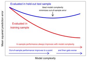
Note: Figure inspired by Figure 7.1 in The Elements of Statistical Learning by Hastie, Tibshirani, and Freedman, which provides a more thorough overview of the problem of overfitting and the bias-variance tradeoff.
How can this be? A classical result in statistics shows that the mean squared prediction error can be decomposed into the bias squared plus the variance. Thus, even if additional predictors reduce the bias in predictions, they can harm predictive performance if they substantially increase the variance of predictions by incorporating random noise.
What can be done?
We have been surprised at how a seemingly small number of variables can yield problems of overfitting in the Fragile Families Challenge. A few ways to combat this problem are:
- Choose a small number of predictors carefully based on theory
- Use a penalized regression approach such as LASSO or ridge regression.
- Use cross-validation to estimate your model’s generalization error within the training set. For an introduction, see chapter 12 of Efron and Hastie [book site]
But at minimum, compare yourself to the baseline to make sure you are doing better than a naive prediction of the mean!
Add your comment