The Fragile Families survey documentation can be confusing. We’ve put together this blog post so you can find out what variables in the Challenge data file mean.

Using the Fragile Families website

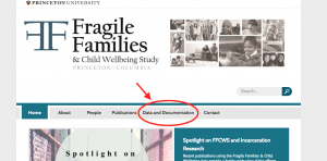
The first place to go to find out what a given variable represents is the Fragile Families and Child Wellbeing Study website: http://www.fragilefamilies.princeton.edu/

Once there, click the “Data and Documentation” tab.

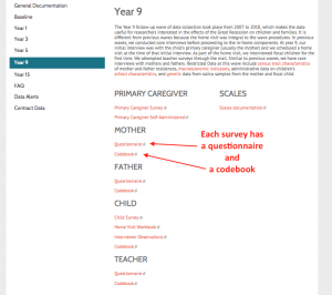
This brings you to the main documentation for the full study. On the left, you will see a set of links that will take you to the documentation for particular waves of the data.

Clicking on the link for Year 9 (Wave 5) as an example, we see the following page of documentation for this survey.

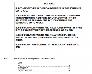
Let’s look at the mother questionnaire and codebook. On page 5 of the questionnaire, you will see the following question:

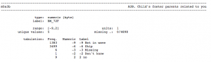
In the corresponding codebook, we see the count of respondents who gave each answer:

Two things are worth noting here.

1. The question referred to in the questionnaire as A3B is called m5a3b in the codebook. This is because the prefix “m5” indicates that this question comes from the mother wave 5 interview.
2. Lot’s of people got coded -6 for “Skip.” Looking back at the questionnaire, we can see why they were skipped over this question: it was only asked of those for whom “PCG = NONPARENT AND RELATIONSHIP = FOSTER CARE.” For children not in foster care, this question would not be meaningful, so it wasn’t asked.

In general, the questionnaires are the best source for information about why certain respondents get skipped over questions. For more information on all the ways data can be missing, see our blog post on missing data.

Structure of the variable names

The general structure of the variable names is [prefix for questionnaire type][wave number][question number].

What are all the variable prefixes?

The most common prefixes are:

Constructed variables: An additional prefix

Some variables have been constructed based on responses to several questions. These are often variable that are particularly relevant to the models many researchers want to estimate. These variables add the additional prefix c to the front of the variable name. For instance, cm1ethrace indicates constructed mother’s wave 1 race/ethnicity.

What are the wave numbers?

It’s easy to talk about the questionnaires by the rough child ages at which they were conducted. This is how the documentation website is organized. However, the variable names always refer to wave numbers, not child ages. It’s important not to get confused on this point. The table below summarizes the mapping between wave numbers and approximate child ages.

What are the question numbers?

Question numbers typically begin with a letter and a number, i.e. a3.

• In questionnaires, questions are referred to by question number alone.
• In codebooks, questions are referred to by a prefix and then a question number.

How do I find a question I care about?

You might want to find a particular question. For instance, when modeling eviction or material hardship at age 15, you might want to include the same measures collected at age 9. If you ctrl+F or cmd+F for “evicted” in the mother or father codebook or questionnaire at age 9, you will find these variables. In this case, they are m5f23d and f5f23d.

GPA measures academic achievement.

We want to know:

• What helps disadvantaged children to beat the odds and succeed academically?
• What derails children so that they perform unexpectedly poorly?

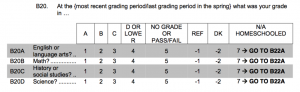
Survey question

How we cleaned the data

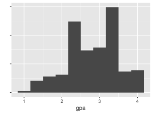
Our measure of GPA is self-reported by the child at approximately age 15. We marked as NA the GPAs of children who were not interviewed, reported no grade, refused to answer, did not know, or were homeschooled, for any of the four subjects. For children with valid answers, we averaged the responses for all four subjects, then subtracted this number from 5 to produce an estimate of child GPA ranging from 1 to 4. In our re-coded variable, a GPA of 4.0 indicates that the child reported straight As, while a GPA of 1.0 indicates that the child reported getting all grades of D or lower.

Distribution in the training set

Scientific motivation

Helping kids “beat the odds” academically is a fundamental goal of education research; academic success can be the key to breaking the cycle of poverty. Free public education is often referred to as a great equalizer, yet children who grow up in disadvantaged families consistently underperform their more affluent peers on average.

However, the average is not the whole story. Some kids do well despite being expected to do poorly. In fact, the amount of unexplained variation in educational achievement is enormous: social science models typically have R-squared values of 0.2 or less [this is based on our informal experience with the literature, not a systematic search]. The poor predictive performance of social science models of educational attainment has long been known. In the now-classic 1972 book Inequality: A Reassessment of the Effect of Family and Schooling in America, Harvard social scientist Christopher Jencks argued that random chance played a larger role than measured family background characteristics in determining socioeconomic outcomes.

While social scientists have learned some about what helps children succeed academically in the decades since 1972, a huge proportion of the variance remains buried in the error term of regression models. Is this term truly random chance, or is there “dark matter” out there in the form of unmeasured but important variables that help some kids to beat the odds?

By submitting a model for GPA at age 15, you help us in our quest to find this dark matter. Based on our collaborative model combining all of the individual submissions, we will identify our best guess as a scientific community about how children are expected to perform at age 15. Then, we will identify a subset of children performing much better and worse than expected. We will interview these children to answer the question: what unmeasured variables are common to the kids who are beating the odds, which we do not observe among the children who are struggling unexpectedly?

When you participate, you help us target interviews at the children whose outcomes are least well explained by our measured variables. These children are best-positioned for exploratory qualitative research to uncover unmeasured but important factors. Interviews may help us learn how some kids beat the odds, these results may drive future deductive research to evaluate the causal effect of these unmeasured variables, and ultimately we hope that policymakers can intervene on the “dark matter” we find in order to improve the lives of other disadvantaged children in the future.

Grit is a measure of passion and perseverance. It predicts success in many domains. The causes of grit remain unknown.

We want to know: What makes some kids unexpectedly grittier than others in adolescence?

Survey questions

The survey questions are adapted from the grit scale proposed by Duckworth, Peterson, Matthews, and Kelly (2007).

How we cleaned the data

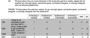
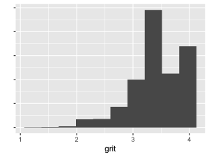
Our measure of grit is based on the four questions above, as answered by the child at approximately age 15. These items were part of a longer battery of questions capturing a wider range of attitudes, emotions, and outlooks. Children who refused any of the four questions or didn’t know how to answer were coded as NA, as were children who did not complete the age 15 interview. For children with four valid answers, we averaged the answers and subtracted the result from 5. This created a continuous scale ranging from 1 to 4. The way we have recoded it, a high score on our variable indicates more grit.

Distribution in the training set

Scientific motivation

Do you keep working when the going gets tough? If so, you probably have a lot of grit.

University of Pennsylvania psychologist and MacArthur “Genius” award winner Angela Duckworth has found that grit predicts all kinds of measures of success: persistence through a military training program at West Point, advancement through the Scripps National Spelling Bee, and educational attainment, to name a few. Duckworth’s work has reached the general public through her TED talk and NY Times bestseller Grit: The Power of Passion and Perseverance.

While it is clear that grit predicts success, it is less clear what causes some people to be grittier than others. How can we help more disadvantaged children to exhibit grit?

A few researchers have begun to examine this question. In their book Coming of Age in the Other America, social scientists Stefanie DeLuca (Johns Hopkins University), Susan Clampet-Lundquist (St. Joseph’s University), and Kathryn Edin (Johns Hopkins University) argue that kids growing up in impoverished urban neighborhoods are often inspired to have grit when they develop passion for an “identity project”: a personal passion that gives them something to aspire toward beyond the challenges of the present day. This ethnographic work exemplifies how qualitative social science research may be able to uncover previously unmeasured sources of grit.

How much more could we learn if qualitative interviews were targeted at the kids best positioned to be informative about unmeasured sources of grit? By participating, you can help us build a community model for grit measured in adolescence. The combined submissions of all who participate will identify our common agreement about the amount of grit we expect to see in the Fragile Families respondents, given all of their childhood experiences from birth to age 9. By interviewing children who have much more or much less grit than we all expect, we will uncover unmeasured factors that predict grit. It is our hope that these unmeasured factors can inform future deductive evaluations and ultimately policy interventions to help kids break the cycle of poverty by developing grit.

Grit is an important predictors of success, but the causes of grit are largely unknown. Be part of the solution and help us target interviews toward those best positioned to show us these unmeasured sources of grit. Apply to participate, build a model, and upload your contribution.

Material hardship is a measure of extreme poverty.

We want to know:

• What helps families to unexpectedly escape extreme poverty?
• What leads families to fall into extreme poverty unexpectedly?

Survey questions

How we cleaned the data

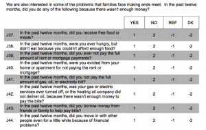
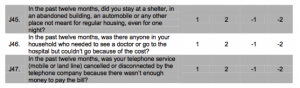
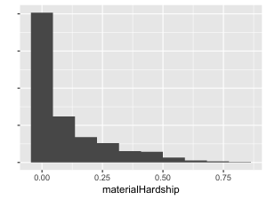
These questions were asked of the child’s primary caregiver when the child was approximately age 15. We marked as NA material hardship for children whose caregivers did not participate in the survey, didn’t know the answer to one or more questions, or refused one or more questions. Our material hardship measure is the proportion of these 11 questions for which the child’s caregiver answered “Yes.” Material hardship ranges from 0 to 1, with higher values indicating more material hardship.

Distribution in the training set

Scientific motivation

In his 1964 State of the Union Address, President Lyndon B. Johnson declared an “all-out war on human poverty and unemployment in these United States.” In the decades since, America has taken great strides toward this goal. However, severe deprivation remains a problem today. In $2 a Day: Living on Almost Nothing in America, Johns Hopkins sociologist Kathryn Edin and University of Michigan social work professor H. Luke Schaefer bring us into the lives of American families living in the nightmare of extreme poverty.

What can be done to reduce extreme poverty? By identifying families who unexpectedly escape extreme poverty, as well as those who unexpectedly fall into it, we hope to uncover unmeasured but important factors that affect severe deprivation.

Measuring extreme poverty is hard. The material hardship scale was originally proposed in a 1989 paper by Susan Mayer and Christopher Jencks, then social scientists at Northwestern University. Rather than focusing solely on respondent’s incomes, Mayer and Jencks asked respondents about particular needs that they were unable to meet. This scale proved fruitful and captured a dimension of poverty above and beyond what was captured by income alone. With minor modifications, the material hardship scale became a standard measure in the federal Survey of Income and Program Participation (SIPP), and it has been included in several waves of the Fragile Families Study.

By participating, you help us to identify the level of material hardship that is expected at age 15 for each of the families in the Fragile Families Study. By combining all of the submissions in one collaborative model, we will produce the best guess by the scientific community of the experiences we expect for families at age 15. Undoubtedly, some families will report much more or much less material hardship than we expect. By interviewing these families, we hope to discover unmeasured but important factors that are associated with sudden dives into material hardship or unexpected recoveries.

The results of these exploratory interviews can then inform future deductive social science research and help us propose policies that could help families to escape severe deprivation. You can help us to target these interviews at the families best positioned to help. Be a part of the solution: apply to participate, build a model, and upload your contribution.

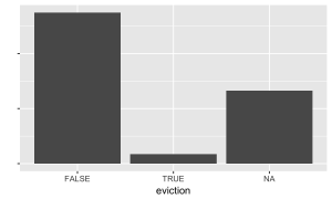
Eviction is a traumatic experience in which families are forced from their homes for not paying the rent or mortgage.

We want to know: As children transition into adulthood, does eviction cause negative outcomes?

Survey question

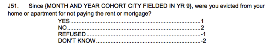
When children were about 15 years old, each child’s primary caregiver was asked the following question:

How we cleaned the data

Those who did not participate in the age 15 interview, as well as those who refused (-1) or didn’t know (-2), were coded as NA. Those who responded “Yes” were coded 1, and those who responded “No” were coded 0. We additionally coded as 1 a small group of respondents who answered in a previous question that they were evicted in the past year, and thus were skipped over this question.

Distribution in the training set

Scientific motivation

In the New York Times bestseller Evicted: Poverty and Profit in the American City, Harvard sociologist and MacArthur “Genius” award winner Matthew Desmond describes fieldwork in which he spent several years living alongside tenants being evicted in low-income Milwaukee neighborhoods. Desmond helped tenants move their things into trucks, followed landlords into eviction court, and watched as children moved from school to school while their families searched for housing. Eviction literally uproots families from their homes, and it is most prevalent among the most disadvantaged urban families. Given Desmond’s qualitative account, it is plausible that eviction may have substantial negative effects on child outcomes in early adulthood.

Emerging evidence further suggests that eviction is sufficiently prevalent to warrant policy attention. Researchers at the Federal Reserve Bank of Atlanta have examined administrative records to find that 12.2 percent of rental households were evicted and forcibly displaced in 2015 in Fulton County, GA (Raymond et al. 2016). Likewise, the Milwaukee Area Renters Study found that 13 percent of private renters experienced a forced move during the 2 years referenced in a survey questionnaire (Desmond and Schollenberger 2015). If eviction creates disadvantage for children, it is sufficiently prevalent to have wide-reaching impacts.

However, untangling cause from selection is no simple task (see our blog post on causal inference and this interview with Matthew Desmond on the topic). It is easy to show that children who experience an eviction have worse outcomes later in life; it is hard to show that these outcomes are not caused by other factors that are correlated with eviction. In a quantitative study using propensity score matching methods on earlier waves of the Fragile Families and Child Wellbeing Study, Desmond and Kimbro (2015) find that eviction is associated with negative outcomes, net of obvious sources of selection bias.

We applaud the work of all the individual research teams that have placed eviction on the table as a scientific concept of interest. However, any individual research team can only adjust for a selected group of observed covariates, and results can be sensitive to the set chosen. We ask you to contribute a model for the probability that a child experiences an eviction between the age 9 and age 15 interviews of the Fragile Families and Child Wellbeing Study, given any set of the birth to age 9 characteristics you choose to include, and any statistical model you choose to employ. Together, we will produce a collaborative propensity score model that the entire scientific community can agree upon, which is not sensitive to researcher decisions. We will then interview a subset of children who are matched on the propensity score, to assess the plausibility of the conditional ignorability assumption required for causal inference (see our blog post on causal inference). If the interview suggest that causal inference may be warranted, we will use these collaborative propensity scores to estimate the causal effect of eviction on child outcomes to be measured several years from now, when children are approximately 22 years old.

In summary, this research agenda will produce estimates of the effect of adolescent eviction on attainment during the transition to adulthood. These collaborative estimates will be robust to the decisions of individual researchers. The assumptions needed for causal inference will be validated in qualitative interviews. These steps will maximize the validity of causal inference in the absence of a randomized experiment.

To achieve these goals, we need your help. Apply to participate, build a model, and upload your contribution!

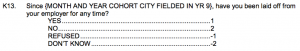
Being laid off is a sudden and often unexpected experience with potentially detrimental consequences for one’s family.

We want to know: When a caregiver is laid off, do adolescent children suffer collateral damage?

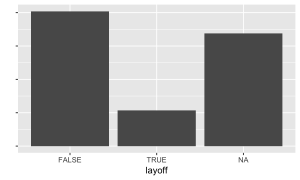
Survey question

When children were about 15 years old, each child’s primary caregiver was asked the following question:

How we cleaned the data

Those who did not participate in the age 15 interview, as well as those who refused (-1) or didn’t know (-2), were coded as NA. Those who have never worked or have not worked since the age 9 interview (in approximately the prior 6 years) were coded as NA; these respondents are not at risk for a layoff. Those who responded “Yes” were coded 1, and those who responded “No” were coded 0.

Distribution in the training set

Scientific motivation

A steady jobs can provide financial security to a family. However, this security can be upset by plant closures, downsizing, and other economic shifts that lead caregivers to lose their jobs. In addition, some caregivers may be fired but report in a survey that they have been laid off. In any case, layoff of a caregiver could create dramatic disadvantages for adolescents nearing the transition to adulthood.

Social scientists worry about layoffs because precarious work is on the rise. In Good Jobs, Bad Jobs, University of North Carolina sociologist Arne L. Kalleberg outlines economic shifts that have made steady employment harder to come by in the United States over the past several decades. Gone are the days when workers could count on a single job to carry them throughout their careers – job changes and unexpected unemployment are now commonplace.

Social scientists also worry about layoffs because they may negatively influence child achievement. Sociologists Jennie E. Brand (UCLA) and Juli Simon Thomas (Harvard) have shown in an article published in the American Journal of Sociology that maternal job displacement reduces a child’s chances of high school and college completion by 3 – 5 percentage points, with even larger effects among those unlikely to experience job displacement and those whose mothers experienced job displacement while the child was an adolescent. When caregivers lose their jobs, children suffer collateral damage.

However, causal conclusions always depend on modeling assumptions. The propensity score matching methods used in the paper cited above assume that the model for the probability of job displacement is correctly specified, and that there are no unmeasured variables that affect job displacement and also directly affect child outcomes. To learn more on these assumptions, see our blog post on causal inference.

The Fragile Families Study follows a particularly disadvantaged sample of urban children, for whom we would especially like to know the effect of maternal layoff on adult outcomes. By participating, you help us to produce a collaborative propensity score model that combines the best of all the individual submissions into a single metric that is robust to the modeling decisions of individual researchers. This model will also help us target interviews at the children best positioned to lend suggestive evidence about the plausibility of the untestable conditional ignorability assumption required for causal inference. If this assumption seems credible after interviews, we will use our collaborative propensity scores to estimate the causal effect of caregiver layoff on child outcomes in early adulthood, once those outcomes are measured several years from now.

By participating, you can be part of an extending our body of knowledge to provide maximally robust causal evidence with observational data about the effect of caregiver layoffs on child outcomes in a disadvantaged urban sample. Results will inform policy changes about whether support for steady caregiver employment could help disadvantaged children.

Be a part of the solution. Apply to participate, build a model, and upload your contribution.

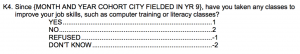
Policymakers often propose programs to retrain the workforce to be able to contribute in a 21st century economy.

We want to know: Do job skills programs utilized by caregivers yield collateral benefits for disadvantaged children?

Survey question

When children were about 15 years old, each child’s primary caregiver was asked the following question:

How we cleaned the data

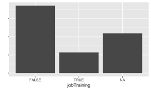
Those who did not participate in the age 15 interview, as well as those who refused (-1) or didn’t know (-2), were coded as NA. Those who responded “Yes” were coded 1, and those who responded “No” were coded 0.

Distribution in the training set

Scientific motivation

One way to raise people’s standard of living is to raise their human capital: the skills that promote productive participation in the labor force. Human capital investments are perhaps more important now than ever before given rapid globalization and computerization of the economy. Does participation in job training programs designed to build computer, language, or other skills improve the well-being of families? When caregivers participate in these programs, do children benefit indirectly?

Social scientists have long been interested in policy interventions to promote employment. This research has also been closely tied to the development of statistical methods for causal inference with observational data. In the 1970s, the National Supported Work Demonstration (NSW) randomly assigned some disadvantaged, non-employed workers to a job training program that included guaranteed employment for a short period of time. Others were randomly assigned to a control condition. The treatment led to measurable increases in earnings in subsequent years, suggesting that job training might be useful.

University of Chicago economist Robert LaLonde saw a new use for these data. Given that experimental results provided the “true” causal effect of job training on earnings, LaLonde wanted to know whether econometric techniques that statistically adjust for selection bias could recover this “true” effect in a non-experimental setting. In general, these statistical adjustments failed to recapture the “true” effect, and LaLonde’s 1986 paper became highly cited as evidence of the extreme difficulty of drawing causal inferences from observational data.

However, the story did not end there. About the same time, a pair of statisticians developed a new method for identifying causal effects: propensity score matching. In an enormously influential 1983 paper, Paul R. Rosenbaum (then of the University of Wisconsin) and Donald B. Rubin (then of the University of Chicago) showed that the average causal effect of a binary treatment on an outcome could be identified by matching treated units with untreated units who had similar probabilities of treatment given observed pre-treatment characteristics. The Rosenbaum and Rubin theorem held only in a sufficiently large sample and only when one estimated the propensity score correctly without omitting any important variables that might affect the treatment and directly affect the outcome. Despite these limitations, the key idea stuck: under certain assumptions, one can use observational data to try to re-create the type of data one would get in a randomized experiment where background characteristics no longer determine treatment assignment.

Empowered with propensity scores, two other statisticians reassessed LaLonde’s findings: could propensity score methods recover the experimental benchmark in the job training example? Raheev H. Dehejia (then of Columbia University) and Sadek Wahba (then of Morgan Stanley) found that they could. In two highly-cited papers (paper 1 and paper 2), they demonstrated that propensity score methods came much closer to recovering the experimental truth than the econometric approaches used by LaLonde.

The saga of job training and causal inference has continued to the present day. For instance, a 2002 paper by economists Jeffrey Smith (then of the University of Maryland) and Petra Todd (University of Pennsylvania) demonstrated that propensity score methods can be highly sensitive to researcher decisions. Since then, numerous statisticians and social scientists have used the job training example to demonstrate the usefulness of new matching methods: entropy balancing (Hainmueller 2012), genetic matching (Diamond and Sekhon 2013), and the covariate balancing propensity score (Imai and Ratkovic 2014), to name a few.

Be part of the next step

Clearly there is a lot of interest in human capital formation through job training. There is also interest in methods to infer causal effects from observational data. How does the Fragile Families Challenge fit in?

A slightly different treatment

The LaLonde (1986) paper and subsequent studies focused on an intensive job training program that connected non-employed individuals with jobs. The “treatment” variable which you will predict is much milder: participation in any classes to improve job skills, such as computer training or literacy classes. Respondents who enroll in these classes are not necessarily non-employed.

A robust propensity score model

One piece of conventional wisdom about propensity score methods is that one should be careful about selecting the pretreatment variables to include in the model, and one must model their relationship to the treatment variable appropriately. This is where you can help! Together we will build a highly robust  community model for the probability of job training. This community model will take all of our best ideas and create one product on which we can all agree.

Specifying models before outcomes occur

A second piece of conventional wisdom of propensity score modeling is that it allows one to conduct all modeling and matching before even looking at the outcome variable. In our case, the ultimate outcome variables are not yet measured: we will examine the effect of caregiver job training on child outcomes in early adulthood. These outcomes will be measured several years from now, long after we lock in our community propensity score model.

Evaluating assumptions

All covariate-adjustment methods to draw causal inferences from observational data rely on the assumption of conditional ignorability (for more about this assumption, see our blog post about causal inference). Through targeted interviews with caregivers, we can provide suggestive evidence as to whether the conditional ignorability assumption holds.

You can help

Be a part of the next step in observational causal inference to evaluate the effect of job training programs. Apply to participate, build a model, and upload your contribution.